Clustering

Clustering consists of receiving an input point cloud and finding points that can be grouped together into clusters. The clusters are typically represented with integer values \(c \in \mathbb{Z}_{\geq -1}\), where the value \(-1\) is used to represent no cluster or noise cluster. Clustering computations are carried out through Clusterer components. They can be included in pipelines. Besides, it is possible to define a post-processing pipeline that will be computed immediately after the clustering.

Clusterers

DBScan clusterer

The DBScanClusterer can be used to compute Density-Based Spatial Clustering of Applications with Noise (DBSCAN) in the point cloud. The DBSCAN algorithm considers a minimum number of points and a radius to define the neighborhood for spatial queries. It finds kernel points, those in whose neighborhood there are at least the minimum number of points. Then, it considers any accessible point to be in the cluster. The accessible points that are not kernel points are included in the cluster because they are close enough to the kernel points. However, these points are not considered to include new points as only kernel points can be used to determine whether a point is accessible or not. The JSON below shows how to define a DBScan clustering component:

{
    "clustering": "fpsdecorated",
    "fps_decorator": {
        "num_points": "m/10",
        "fast": true,
        "num_encoding_neighbors": 1,
        "num_decoding_neighbors": 1,
        "release_encoding_neighborhoods": false,
        "threads": 16,
        "representation_report_path": null
    },
    "decorated_clusterer": {
        "clustering": "dbscan",
        "cluster_name": "cluster_wood",
        "precluster_name": "prediction",
        "precluster_domain": [1],
        "min_points": 200,
        "radius": 3.0,
        "post_clustering": [
            {
                "post-processor": "ClusterEnveloper",
                "envelopes": [
                    {
                        "type": "AlignedBoundingBox",
                        "compute_volume": true,
                        "output_path": "*/aabbs.csv",
                        "separator": ","
                    },
                    {
                        "type": "BoundingBox",
                        "compute_volume": true,
                        "output_path": "*/bboxes.csv",
                        "separator": ","
                    }
                ]
            }
        ]
    }
}

The JSON above defines a DBScanClusterer that is decorated to work on a FPS representation of the input point cloud (see the FPS decorated clusterer documentation for further details). It will consider all the points predicted as wood to compute clusters of wood. The minimum number of points in the neighborhoods of kernel points is set to 200 points, and the radius of the neighborhood to 3 meters. After computing the clustering, a post-processing pipeline will be run to find the axis-aligned and oriented bounding boxes, respectively. For each bounding box the vertices, the cluster label, and the enclosed volume will be exported to a CSV file using , as separator.

Arguments

– cluster_name: The name of the clusters. For instance, when finding clusters of buildings it is a good idea to use "cluster_building" as the cluster name.
– precluster_name: In case the point cloud is already clustered, the precluster name specifies the point-wise attribute to consider to filter the points. Note that both reference and predicted classes can be seen as clusters.
– precluster_domain: If the preclustering filter is applied, then the precluster domain list can be used to specify the values of interest (any point that is not in the domain will be ignored). If not given and preclustering filter is requested, then the precluster domain will be automatically inferred as the set of unique values for the attribute.
– min_points: The minimum number of points that must belong to a neighborhood to pass the kernel point check.
– radius: The radius of the neighborhood for kernel point checks.
– post_clustering: The post-clustering pipeline. It can be null or a list of post-clustering components.

Bivariate critical clusterer

The BivariateCriticalClusterer can be used to compute one cluster per critical point in the given point cloud. The bivariate critical clustering algorithm considers the requested type of critical point (e.g., min or max) and then does a distance-based clustering. It is called bivariate because it works on three variables \((x, y, z)\) (they can be the coordinates or any other variables, including those from the feature space). Assuming Monge form \(z = \hat{z}(x, y)\), the critical points will correspond to the minima or maxima of the third variable \(z\) on the surface defined by the other two \((x, y)\). The clusters for each critical point can be computed through the nearest neighbor method or using a distance-based region growing algorithm. The JSON below shows how to define a bivariate critical clustering component:

{
    "clustering": "BivariateCritical",
    "cluster_name": "avocado",
    "precluster_name": "prediction",
    "precluster_domain": [1],
    "critical_type": "max",
    "filter_criticals": false,
    "radius": 2.0,
    "x": "x",
    "y": "y",
    "z": "z",
    "strategy": {
        "type": "RecursiveRegionGrowing",
        "initial_radius": 0.25,
        "growing_radius": 0.25,
        "max_iters": 20000,
        "first_stage": false,
        "first_stage_correction": false,
        "second_stage": true,
        "nn_correction": false
    },
    "label_criticals": false,
    "critical_label_name": "max",
    "chunk_size": 50000,
    "nthreads": 8,
    "kdt_nthreads": 2
}

The JSON above defines a BivariateCriticalClusterer that will consider the point-wise coordinates (i.e., the structure space of the point cloud) as the variables for the clustering. The critical points will be searched on a radius of \(2\) meters and the clustering strategy will be the recursive region growing algorithm. Furthermore, the clustering will be computed in parallel dividing the workload in chunks of \(50,000\) points using \(8\) parallel jobs, each with \(2\) threads for each KDTree-based spatial query.

Arguments

– cluster_name

The name of the clusters. For instance, when finding clusters of avocados it is a good idea to use "avocado" as the cluster name.

– precluster_name

In case the point cloud is already clustered, the precluster name specifies the point-wise attribute to consider to filter the points. Note that both reference and predicted classes can be seen as clusters.

– precluster_domain

If the preclustering filter is applied, then the precluster domain list can be used to specify the values of interest (any point that is not in the domain will be ignored).

– crtical_type

The type of critical point to be considered, either "min" or "max".

– filter_criticals

Boolean mask governing whether to filter critical points in case there is more than one in a neighborhood of the given radius. When true all the crtitical points in the same neighborhood but one will be discarded (this happens when both are maxima or minima, e.g., they have the same \(z\) coordinate). When false all the critical points will be kept, even if this implies more than one per neighborhood.

– radius

The radius for the neighborhood analysis used to find the critical points. Note that it is a 2D radius because only the first and second variables (i.e., \((x, y)\)) are considered for the spatial queries.

– x

The first variable, e.g., "x".

– y

The second variable, e.g., "y".

– z

The third variable, e.g., "z". Note that critical points will be minima or maxima with respect to this variable.

– strategy

The strategy specification for the clustering. It can be either the nearest neighbor method or the recursive region growing algorithm.

– Nearest neighbor method

– type

It must be "NearestNeighbor".

– Recursive region growing algorithm

– type

It must be "RecursiveRegionGrowing".

—initial_radius

The radius for the initial clusters. The distance is computed considering the \((x, y)\) variables, i.e., in 2D. All the points that are inside this radius with respect to a critical point will belong to its cluster.

—growing_radius

The radius for each region growing step. Again, distances will be computed in the plane defined by the first two variables \((x, y)\).

—max_iters

The maximum number of iterations for the clustering. If zero, then the clustering will run until full convergence is achieved.

—first_stage

Whether to compute the first stage of the region growing strategy (true) or not (false). This stage considers any point in the cluster to analyze its neighborhood. Any point in the neighborhood that is at the same height or lower (when max critical points are considered) or at the same height or above (when min critical points are considered) will be included in the cluster. The aforementioned process will be computed recursively until not more points are added to a cluster or the max number of iterations is reached.

—first_stage_correction

Whether to apply a concave hull-based correction to the first stage (true) or not (false). The correction consists of computing the 2D concave hull for each cluster (on the \(x\) and \(y\) coordinates) and then include in the cluster any point that is inside the concave hull.

—second_stage

Whether to compute the second stage of the region growing strategy. In this stage, the clusters grow considering the neighborhood for each point in the cluster, and doing so recursively to account for newly added points during the iterations of the second stage too. The second stage stops when not even a single cluster grew or when the maximum number of iterations is reached.

—nn_correction

Whether to apply the nearest neighbor method after finishing the clustering (true) or not (false). If applied, it will consider all the points that have not been clustered by the region growing algorithm and assign them to the cluster of its closest clustered neighbor.

– label_criticals

Whether to label the critical points (true) or not (false). Note that the point cloud will be updated with an extra feature that will be a label specifying whether it is a critical point or not.

– critical_label_name

The name for the feature that labels critical points.

– chunk_size: How many points per chunk for the parallel exeuction. If zero, then all the points are consireded in a single chunk.
– nthreads: How many chunks will be computed in parallel at the same time.
– kdt_nthreads: How many threads will be used to speedup the computation of the spatial queries through the KDTree. Note that the final number of parallel jobs will be \(\text{nthreads} \times \text{kdt_nthreads}\).

Output

The figure below represents the bivariate critical clusters computed on the maxima of a previously classified avocado plantation. There are approximately as many clusters as avocados, with each cluster generally corresponding to a different avocado.

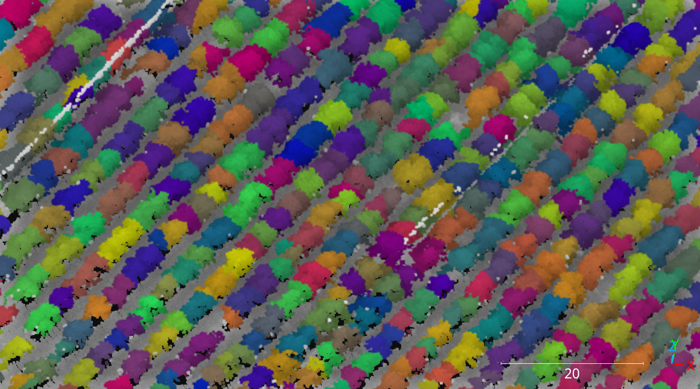
Figure representing avocado cluster. — Visualization of the avocado clusters computed through the bivariate critical clustering algorithm with the region growing strategy.

Simple features clusterer

The SimpleFeaturesClusterer can be used to compute clusters by filtering points considering relational conditions. These relationals can be specified similar to how it is done for the cluster selector post-processor. The JSON below shows how to define a simple features clusterer:

{
    "clustering": "SimpleFeatures",
    "cluster_name": "change_cluster",
    "cluster_value": 1,
    "filters": [
        {
            "attribute": "chg_euclid",
            "relational": "greater_than_or_equal_to",
            "target": 0.33,
            "action": "preserve"
        }
    ]
}

The JSON above defines a SimpleFeaturesClusterer that makes a cluster with all the points that have Euclidean distance-based point-wise change quantification greater than \(0.33\) meters. The points that do not belong to the cluster will have a value of zero, those that belong to the cluster will have a value of one. The name of the feature representing the cluster is "change_cluster".

Arguments

– cluster_name: The name of the feature representing the cluster.
– cluster_value: The value for the points that belong to the cluster.
– filters: See cluster selector filters documentation.

Simple curve extractor

The SimpleCurveExtractor extracts clean, parameterized 3D curves from previously classified or clusterized point clouds. It implements a 6-stage pipeline: adaptive stabilization, soft 2.5D skeleton extraction, monotonic topological pruning, resilient geometry refinement, multi-format output, and optional reverse label propagation. The JSON below shows how to define a simple curve extractor:

{
    "clustering": "SimpleCurveExtractor",
    "cluster_name": "CURVE",
    "curve_source": "classification",
    "curve_classes": [4],
    "min_voxel_size": 0.1,
    "merge_radius": 15.0,
    "z_tolerance": 2.0,
    "min_segment_length": 3.0,
    "spatial_scale": 1.5,
    "min_curve_length": null,
    "min_twig_length": null,
    "rdp_tolerance": null,
    "curve_pcloud_step": null,
    "snap_densify_step": null,
    "snap_max_shift": null,
    "snap_target_radius": null,
    "snap_pull_radius": null,
    "hallucination_drop_densify_step": null,
    "hallucination_drop_radius": null,
    "hallucination_min_supported_length": null,
    "endpoint_extension_step": null,
    "endpoint_extension_radius": null,
    "endpoint_extension_max_length": null,
    "cid_relabel_z_disjoint_threshold": null,
    "cid_gap_split_dz_threshold": null,
    "max_merge_iterations": 3,
    "tangent_smoothing_iterations": 3,
    "occupancy_threshold": 0.1,
    "chain_radius_factor": 3.0,
    "angular_threshold_k": 1.5,
    "betweenness_percentile": 0.05,
    "ridge_fraction": 0.5,
    "output_point_spacing": 0.0,
    "z_consistency_sigma": 0.0,
    "snap_enable": true,
    "snap_min_neighbors": 4,
    "snap_smoothing_iterations": 2,
    "snap_passes": 30,
    "snap_post_passes": 20,
    "hallucination_drop_enable": true,
    "hallucination_drop_threshold": 0.025,
    "snap_truncate_iterations": 15,
    "endpoint_extension_enable": true,
    "cid_relabel_z_disjoint_enable": true,
    "cid_gap_split_enable": true,
    "cid_gap_split_planar_radius": 15.0,
    "merge_orphans_enable": true,
    "final_cleanup": false,
    "slope_output_form": "angle_deg",
    "propagate_labels": true,
    "curve_pcloud": "*/curve_pcloud.las",
    "output_gpkg": "*/break_curves.gpkg",
    "output_shp": "*/break_curves.shp",
    "output_csv": "*/break_curves.csv",
    "epsg": 25829,
    "nthreads": -1,
    "post_clustering": null
}

The JSON above defines a SimpleCurveExtractor that will extract 3D curves from points classified as class \(3\) (e.g., roads). The adaptive stabilization will run up to \(3\) merge iterations with \(3\) tangent smoothing iterations. The skeleton will be extracted using a z_tolerance of \(2.0\) (soft-Z sigma) and an occupancy threshold of \(0.1\). Topological pruning removes twigs shorter than \(50 \times \text{min_voxel_size}\) (i.e. \(5.0\) m at the default voxel size) and prunes low-centrality edges below the \(5\)-th percentile. The final geometry is simplified with an RDP tolerance derived from min_voxel_size (\(0.1\) m by default). Extracted curves will be exported to GeoPackage, Shapefile, and CSV formats in the EPSG:25830 coordinate reference system. Computations will use all available cores.

Example configuration notes:

All hidden/advanced kwargs are listed at their default values so the JSON above can be used as a “copy this, customise the line you care about” template.
rdp_tolerance and min_twig_length use the sentinel null. When omitted (or null) they are derived from min_voxel_size so they track the input coordinate scale (see their individual argument entries for the derivation).
snap_densify_step, hallucination_drop_densify_step, and endpoint_extension_step likewise use the sentinel null. When unset they each resolve to \(5 \times \text{min_voxel_size}\) (i.e. \(0.5\) m at the default voxel size), matching the densification step on the production fixture.
cid_gap_split_planar_radius also defaults to null and resolves to merge_radius when the latter is set. If merge_radius is itself null it falls back to the default \(15.0\) m so the gap-split pass keeps its metric-aligned planar radius.

Note

Some kwargs use the sentinel null and resolve at instance construction to a fixed coefficient times min_voxel_size so the algorithm scales with the input voxel resolution.

min_twig_length – \(50 \times \text{min_voxel_size}\)
(= \(5.0\) m at default).
rdp_tolerance – \(\text{min_voxel_size}\)
(= \(0.1\) m at default).
min_curve_length – \(500 \times \text{min_voxel_size}\)
(= \(50.0\) m at default).
curve_pcloud_step – \(1 \times \text{min_voxel_size}\)
(= \(0.1\) at default).
snap_densify_step – \(5 \times \text{min_voxel_size}\)
(= \(0.5\) m at default).
snap_max_shift – \(35 \times \text{min_voxel_size}\)
(= \(3.5\) m at default).
snap_target_radius – \(30 \times \text{min_voxel_size}\)
(= \(3.0\) m at default).
snap_pull_radius – \(400 \times \text{min_voxel_size}\)
(= \(40.0\) m at default).
hallucination_drop_densify_step – \(5 \times \text{min_voxel_size}\)
(= \(0.5\) m at default).
hallucination_drop_radius – \(25 \times \text{min_voxel_size}\)
(= \(2.5\) m at default).
hallucination_min_supported_length – \(1 \times \text{min_voxel_size}\)
(= \(0.1\) m at default).
endpoint_extension_step – \(5 \times \text{min_voxel_size}\)
(= \(0.5\) m at default).
endpoint_extension_radius – \(25 \times \text{min_voxel_size}\)
(= \(2.5\) m at default).
endpoint_extension_max_length – \(150 \times \text{min_voxel_size}\)
(= \(15.0\) m at default).
cid_relabel_z_disjoint_threshold – \(50 \times \text{min_voxel_size}\)
(= \(5.0\) m at default).
cid_gap_split_dz_threshold – \(30 \times\text{min_voxel_size}\)
(= \(3.0\) m at default).

Arguments

Input configuration

– curve_source: The source attribute from which curve points are selected. It can be "classification" to use the point cloud’s classification attribute, "predictions" (or equivalently "prediction") to use predicted labels, or any custom attribute name to access an extra dimension by name from the LAS structure. The three built-in keywords ("classification", "prediction", "predictions") are matched case-insensitively; a custom attribute name is passed through verbatim to the LAS-dimension lookup and is therefore case-sensitive. When the predictions array is two-dimensional and of a floating-point dtype (i.e. per-class probabilities), hard labels are derived via \(\operatorname{argmax}\) along the class axis.
– curve_classes: A list of integer class or cluster IDs that identify curve points. All points whose curve_source attribute matches one of these values will be used as input for the curve extraction pipeline.

Stage 1: Adaptive stabilization

– max_merge_iterations: The maximum number of convergence iterations for the adaptive stabilization stage. During each iteration, disconnected endpoint pairs are scored and merged when their combined distance, tangent alignment, and component size score exceeds the acceptance threshold. Default is \(3\).
– tangent_smoothing_iterations: The number of iterations for tangent field smoothing within the stabilization stage. Higher values produce smoother tangent estimates at the cost of reduced locality. Default is \(3\).
– min_voxel_size: The minimum allowed voxel size for adaptive voxelization. Prevents pathological cases where duplicate points or noise produce an extremely small median nearest-neighbor distance. The actual voxel size is computed as \(V = \max(1.5 \times \text{median_nn}, \text{min_voxel_size})\). min_voxel_size also acts as the reference scale for several scale-coupled downstream thresholds (min_twig_length, rdp_tolerance, the \(\Delta z_{\max}\) floor, and the Z-jump bridge floor), so pick a value consistent with the input coordinate scale. Default is \(0.1\).

Stage 2: Soft 2.5D skeleton extraction

– z_tolerance

Soft-Z sigma \(\sigma_z\) used by the occupancy weighting. It controls the Gaussian weighting of point heights when building the 2.5D occupancy grid: \(\text{occupancy}(\text{cell}) = \sum_i \exp\left(-\frac{(Z_i - Z_{\text{ref}})^2}{2\,\sigma_z^2}\right)\). This parameter also governs the maximum Z-difference threshold \(\Delta z_{\max}\) used by the cylindrical merge criterion and the three Z-artifact detectors (bridge Z-jump split, vertical column split, Z-reversal split; see merge_radius). Default is \(2.0\).

– occupancy_threshold

The binary threshold applied to the soft-Z occupancy values. Cells with occupancy below this threshold are considered unoccupied. Default is \(0.1\).

– spatial_scale

The skeleton-extraction voxel size, independent of the stabilization voxel size. When set to \(0.0\) (default), the stabilization voxel size is used. For wide curves (e.g., roads), setting this to a value larger than the default (e.g., \(1.0\)–\(2.0\) meters) produces cleaner centerlines by reducing the skeleton grid resolution.

– merge_radius

The endpoint merge radius. When set (not null), endpoint pairs are tested against a cylindrical proximity criterion: the 2D (XY-plane) distance must be within the merge radius \(r_m\), and the absolute Z-difference must not exceed a maximum threshold \(\Delta z_{\max}\):

\[\| \mathbf{p}_a^{xy} - \mathbf{p}_b^{xy} \|_2 \;\le\; r_m \qquad\text{and}\qquad | z_a - z_b | \;\le\; \Delta z_{\max}\]

where the Z-difference threshold is derived from z_tolerance:

\[\Delta z_{\max} = \max\!\bigl(\min(3\,\sigma_z,\; r_m),\; 10 \times \text{min_voxel_size}\bigr)\]

The \(\max(\cdot,\, 10\,V_{\min})\) floor prevents degenerate behaviour when \(\sigma_z = 0\) and scales with min_voxel_size so the threshold is portable across coordinate scales (metre, sub-metre, or very-large clouds). At the default min_voxel_size = 0.1 the floor is \(1\,\text{m}\), matching the legacy metre-scale behaviour. This cylindrical test is used in three stages: endpoint merging (connecting different curve components), post-chain merging (reconnecting same-curve segments), and post-resolve merging (reconnecting endpoints created by cross-feature truncation).

Three post-processing artifact detectors are derived from \(\Delta z_{\max}\) to remove elevation artifacts produced by multi-terrace skeleton connections:

Bridge Z-jump split. Operates on each polyline using the consecutive XY spacings \(\Delta xy_k\) and their median \(\widetilde{\Delta xy}\). A segment \(k\) is flagged as a Z-jump bridge when either of two criteria holds.

The moderate-bridge criterion flags short gaps with a large vertical jump:

\[\Delta xy_k > \max\!\bigl(3\,\tilde{\Delta xy},\; 10 \times \text{min_voxel_size}\bigr) \quad\text{and}\quad |\Delta z_k| > \max\!\left( \frac{\Delta z_{\max}}{2},\; 1\right)\]

The \(\max(\cdot, 10\,V_{\min})\) XY floor and the \(\max(\cdot, 1)\) Z floor prevent degenerate thresholds when the polyline is very tight or \(\Delta z_{\max}\) is small. The Z floor of \(1\) is an absolute constant from the code and does not scale with min_voxel_size.

The long-bridge criterion flags long gaps with a moderate vertical jump:

\[\Delta xy_k > \ell_{xy} \quad\text{and}\quad |\Delta z_k| > \ell_z\]

where the thresholds track the pipeline’s spatial and Z-noise scales:

\[\begin{split}\ell_{xy} = \begin{cases} \tfrac{2}{3}\,r_m & \text{if } r_m > 0 \\ 10 & \text{otherwise} \end{cases} \qquad \ell_z = \begin{cases} \sigma_z & \text{if } \sigma_z > 0 \\ 2 & \text{otherwise} \end{cases}\end{split}\]

At the legacy test defaults (\(r_m = 15\), \(\sigma_z = 2\)) these recover \(\ell_{xy} = 10\,\text{m}\) and \(\ell_z = 2\,\text{m}\).

Flagged indices split the polyline into independent sub-features; the short arc immediately surrounding the jump is then removed by the min_curve_length / short-curve-artifact filter downstream.
Vertical column split. A windowed grade analysis detects contiguous runs where Z changes rapidly relative to 2D movement. Let \(N\) be the number of polyline vertices and \(w = \min(100,\, \lfloor N/4 \rfloor)\); the detector is only engaged when \(w \ge 10\). For each window start \(i\) the grade is

\[G_w(i) = \frac{|z_{i+w} - z_i|} {\max\!\bigl(\sum_{k=i}^{i+w-1} \Delta xy_k,\; 0.1\bigr)}\]

Let \(I = \{i : G_w(i) > \tan(\theta)\}\) be the set of vertical-grade hits. Consecutive hits are grouped into runs: two successive indices \(i_j,\, i_{j+1} \in I\) belong to the same run when \(i_{j+1} - i_j \le w\); a gap \(> w\) starts a new run. For each run the polyline is split both at the run-start index \(i_{\text{start}}\) and at \(i_{\text{end}} + w\) (clamped to the polyline’s interior), so the vertical column is isolated as a short sub-feature the downstream min_curve_length / short-curve-artifact filter then drops. Here \(\theta\) is fixed at \(\pi/4\) (giving \(\tan(\theta) = 1\) — steeper than \(45^{\circ}\)).
Z-reversal split. A drawdown analysis detects features whose elevation profile climbs to an interior peak and then drops by more than \(\Delta z_{\max}\):

\[D(i) = \max_{j \le i} z_j \;-\; z_i \qquad\Longrightarrow\qquad \text{split where } D(i) > \Delta z_{\max}\]

The feature is split at the peak preceding the excessive drawdown. Peaks at the very start or end of the feature (monotonic descents) are not considered reversals.

When null (default) or set to a non-positive value, no merging or artifact splitting is performed — the internal enable flag is merge_radius is not None and merge_radius > 0.

Stage 3: Monotonic topological pruning

Stage 3 operates on the skeleton graph \(G = (V, E)\) produced by Stage 2 — an undirected radius graph whose nodes are the extracted skeleton points and whose edges connect skeleton points that were judged topologically adjacent. Given a node \(i \in V\), we write \(\deg(i)\) for its degree (the number of edges incident to \(i\) in \(E\)) and \(\mathcal{N}(i)\) for its neighbor set; these are the only graph primitives the rest of the stage relies on. Stage 3 runs four sequential operations — twig pruning, junction detection, betweenness-based chain pruning, and cycle validation — each of which consumes the output of the previous step.

– min_twig_length

Minimum length (in point-cloud units) of a twig — a chain of degree-2 nodes emanating from a degree-1 endpoint — below which the twig is removed. Twig tracing, implemented in TopologicalPruner::pruneTwigs, starts from every node \(e\) with \(\deg(e) = 1\) and walks the unique chain \(e = v_0 \to v_1 \to \dots \to v_m\) through degree-2 nodes, stopping at the first stop node — either a junction (flagged by angular_threshold_k below), a graph boundary, or another degree \(\ne 2\) node. The twig length is its cumulative Euclidean arc length

\[L(v_0,\dots,v_m) = \sum_{k=0}^{m-1} \bigl\lVert \mathbf{x}_{v_{k+1}} - \mathbf{x}_{v_k}\bigr\rVert_2.\]

If \(L < \text{min_twig_length}\), every edge along the chain is removed from \(G\). Chains whose both endpoints are degree-1 are deduplicated (traced once) so they are not removed twice.

When set to null (default) the value is derived as \(50 \times \text{min_voxel_size}\) (i.e. \(5.0\) at the default \(\text{min_voxel_size} = 0.1\)). The sentinel is resolved in __init__() and the derived value is what pruneTwigs actually receives.

– angular_threshold_k

Robust multiplier \(k\) that selects which high-degree nodes are classified as junctions. The detector, in TopologicalPruner::detectJunctions, proceeds as follows.

Candidate set. Let \(C = \{ i \in V : \deg(i) \ge 3 \}\) be the set of candidate nodes. A degree-1 or degree-2 node cannot express branching, so it is never a junction candidate.
Per-node angular spread. For each candidate \(i \in C\), compute the unit directions from \(i\) to each of its neighbors,

\[\mathbf{d}_{i \to j} = \frac{\mathbf{x}_j - \mathbf{x}_i} {\lVert \mathbf{x}_j - \mathbf{x}_i\rVert_2}, \qquad j \in \mathcal{N}(i),\]

(neighbors at exactly the same position as \(i\) are discarded via a \(10^{-12}\) length check). The angular spread \(\alpha(i)\) is the maximum pairwise angle among those unit directions:

\[\begin{split}\alpha(i) = \max_{\substack{ j_1, j_2 \in \mathcal{N}(i) \\ j_1 < j_2}} \arccos\!\bigl( \mathbf{d}_{i \to j_1} \cdot \mathbf{d}_{i \to j_2} \bigr).\end{split}\]

The dot product is clamped to \([-1, 1]\) before the \(\arccos\) to absorb floating-point drift. Candidates with fewer than two finite unit directions receive \(\alpha(i) = 0\).
Robust global threshold. Let \(m = \operatorname{median}_{i \in C}\alpha(i)\) and

\[s = \operatorname{median}_{i \in C} \bigl|\alpha(i) - m\bigr|\]

be the median and median absolute deviation (MAD) of the candidate spreads. The junction threshold is

\[\tau_{\alpha} = m + k \cdot s.\]

Using the MAD rather than the standard deviation makes \(\tau_{\alpha}\) robust to a handful of extreme Y-shaped splits that would otherwise inflate a mean/stddev estimate.
Flagging. A candidate \(i \in C\) is marked as a junction iff \(\alpha(i) > \tau_{\alpha}\). The resulting junction mask is consumed by pruneTwigs (stop criterion) and by the segment/curve-ID assignment downstream.

Raising \(k\) makes the threshold stricter and produces fewer junctions — more branches are then treated as plain degree-2 chain vertices. Default is \(1.5\).

– betweenness_percentile

Percentile cutoff \(p \in [0, 1]\) on edge betweenness centrality. For an undirected graph, Brandes’ (2001) unweighted edge betweenness is

\[\begin{split}c_B(e) = \sum_{\substack{s, t \in V \\ s \ne t}} \frac{\sigma_{st}(e)}{\sigma_{st}},\end{split}\]

where \(\sigma_{st}\) is the number of shortest paths from \(s\) to \(t\) and \(\sigma_{st}(e)\) is the number of those paths that traverse edge \(e\). Shortest is measured by hop count: every edge has unit length. Intuitively, \(c_B(e)\) counts how often \(e\) appears on a shortest path between arbitrary pairs of nodes — bridge-like edges on the backbone of \(G\) score high, peripheral side-roads score low.

Brandes’ algorithm computes all \(c_B(e)\) in \(O(|V|\,|E|)\) total. For each chosen source \(s \in V\), a single breadth-first search (BFS) from \(s\) populates four arrays over nodes \(v \in V\):

\(d_s(v)\) — the number of edges on a shortest \(s \to v\) path;
\(\sigma_s(v)\) — the count of shortest \(s \to v\) paths, accumulated during the BFS layer sweep via \(\sigma_s(w) \mathrel{+}= \sigma_s(v)\) whenever \(d_s(w) = d_s(v) + 1\) and \(w \in \mathcal{N}(v)\);
\(P_s(v)\) — the list of predecessors of \(v\) on its shortest paths from \(s\);
\(\delta_s(v)\) — the source-dependent dependency of \(v\), computed bottom-up after the BFS in decreasing-\(d_s\) order by

\[\delta_s(v) = \sum_{w : v \in P_s(w)} \frac{\sigma_s(v)}{\sigma_s(w)} \bigl(1 + \delta_s(w)\bigr).\]

The edge dependency contributed by source \(s\) to edge \((v, w)\) with \(v \in P_s(w)\) is \((\sigma_s(v)/\sigma_s(w))\,(1 + \delta_s(w))\), and the final edge centrality is the sum over all chosen sources \(s\). (Breadth-first search, BFS, is the canonical graph traversal that visits all nodes at hop distance 1 from the source first, then all at hop distance 2, and so on; it yields shortest-path distances in unweighted graphs in \(O(|V| + |E|)\) per source.)*

Where the centrality is computed. Running Brandes’ on the raw skeleton graph is wasteful because every degree-2 chain adds redundant edges that all carry the same score. Stage 3 therefore first contracts the graph: each maximal degree-2 chain between two non-degree-2 endpoints \(a, b\) collapses to a single edge \((a, b)\) in a contracted graph \(\tilde{G}\), with that edge’s weight irrelevant for the BFS (edges are still unit-length during the shortest-path computation). Centrality is then computed on \(\tilde{G}\), the score of each contracted edge is mapped back to all the original edges along the corresponding chain, and the pruning threshold is applied in the original graph.

Pruning. Let \(c_{(1)} \le c_{(2)} \le \dots \le c_{(M)}\) be the contracted-edge scores sorted ascending (one score per contracted edge, \(M\) = contractedChainCount). The code selects the threshold index

\[\operatorname{pIdx} = \lfloor p \cdot (M-1) \rfloor \in \{0, 1, \dots, M-1\},\]

(0-based, clamped to \(M-1\)) and sets \(\tau_B = c_{(\operatorname{pIdx} + 1)}\) (1-based order statistic), which is the standard left-tail percentile estimate for sample size \(M\). Every original edge whose corresponding contracted edge has score \(c \le \tau_B\) is removed from \(G\).

The \(\le\) comparison has two notable edge cases:

\(p = 0\) does not disable the prune. With \(\operatorname{pIdx} = 0\), \(\tau_B = c_{(1)} = \min_i c_i\), so the minimum-score edge is removed and all other edges tied with that minimum are removed as well. In a graph with no ties at the minimum, exactly one contracted edge (and all original edges it represents) is pruned per pass.
\(p = 1\) gives \(\tau_B = c_{(M)} = \max_i c_i\), so every contracted edge satisfies \(c \le \tau_B\) and the entire backbone is stripped. This is degenerate and is not a supported operating point.

With \(p = 0.05\) (default), roughly the bottom 5 % of backbone edges are pruned each pass. Default \(p = 0.05\).

– ridge_fraction

Relative distance-transform (DT) threshold used to validate (or break) cycles in the pruned graph. Each skeleton node \(v\) inherits from Stage 2 a scalar DT value \(dt(v) \ge 0\) produced by the exact Felzenszwalb-Huttenlocher 2D Euclidean Distance Trasnsform (EDT) on the soft-Z binary occupancy grid. The EDT is seeded on background (unoccupied) cells (the standard medial-axis convention), so if \(\mathrm{cell}(v)\) is the 2D voxel containing \(v\) and \(B\) is the set of background cells of the pre-thinning occupancy grid, each cell \(q\) is assigned

\[E^2(q) = \min_{p \in B}(q - p)^2,\]

and the per-node DT is

\[dt(v) = \sqrt{E^2\!\bigl(\mathrm{cell}(v)\bigr)} \cdot V,\]

where \(V\) is the voxel size. The validateCycles helper consumes these values verbatim. Because skeleton nodes are, by construction, interior points of the occupied region surviving Zhang-Suen thinning, they sit at positive \(dt\): thick medial ridges carry large values, boundary-adjacent nodes carry small ones. A genuine ridge-like curve therefore has uniformly high \(dt\) along its length; spurious loops closed across narrow chokepoints contain at least one node whose \(dt\) is comparatively small.

Let \(m_{dt} = \operatorname{median}_{v \in V} dt(v)\) and define the global DT threshold

\[\tau_{dt} = \text{ridge_fraction} \cdot m_{dt}.\]

Cycles are discovered by an iterative (stack-based) depth-first traversal of the currently active subgraph (\(\deg(v) > 0\) nodes). The implementation does not maintain the classical discovery/finish-time coloring, so “back edge” here is a DFS-tree heuristic: an edge \((u, v)\) examined during traversal is flagged when

\[v \in \operatorname{visited} \quad\text{and}\quad v \neq \operatorname{parent}(u) \quad\text{and}\quad \operatorname{depth}(v) < \operatorname{depth}(u),\]

i.e. it re-enters an already-visited node that is not the parent in the DFS tree and that lies at a strictly smaller DFS depth. On a plain undirected graph traversed with an explicit stack this captures the typical cycle-closing edges without the overhead of the two-color scheme. Let \(C\) be the cycle this back edge closes, reconstructed by walking the DFS parent pointers from \(u\) back to \(v\). The cycle is characterised by its minimum edge DT

\[\operatorname{minDT}(C) = \min_{(a, b) \in C} \min\!\bigl(dt(a),\, dt(b)\bigr),\]

i.e. the DT of the weakest edge along \(C\) (edge DT is defined as the minimum of its two endpoint DTs). If \(\operatorname{minDT}(C) < \tau_{dt}\) the cycle is flagged as spurious — at least one of its edges is too close to the boundary to represent a real loop — and the weakest edge of \(C\) (the \((a, b) \in C\) achieving the \(\operatorname{minDT}\)) is removed, breaking the cycle. If \(\operatorname{minDT}(C) \ge \tau_{dt}\), the cycle is preserved.

Raising ridge_fraction makes \(\tau_{dt}\) larger relative to the median, so more cycles fail the check and are broken; lowering it preserves more cycles. With the default \(0.5\), a cycle must have every edge at DT no smaller than half the median nodal DT to survive.

Operating regime. Zhang-Suen thinning preserves only cells that retain at least one background neighbour, so every surviving skeleton cell is at squared cell-distance \(\ge 1\) from the nearest background cell. Scaled by the voxel size this gives a hard lower bound

\[\min_{v} dt(v) \;\ge\; V,\]

i.e. the smallest per-node DT is at least the voxel size \(V\) (spatial_scale when set, otherwise the Stage-1 adaptive voxel size). Because \(\tau_{dt} = \text{ridge\_fraction} \cdot m_{dt}\) must exceed \(\min_v dt(v) \ge V\) for any cycle edge to qualify for removal, the effective no-fire threshold is

\[\text{ridge\_fraction} \;\lesssim\; \frac{V}{m_{dt}}.\]

On typical breakline inputs \(m_{dt}\) sits roughly at \(1.4\,V\) (so \(V / m_{dt} \approx 0.7\)), which means the documented default \(0.5\) is effectively a no-op for cycle validation on those inputs — the step becomes active only once \(\text{ridge\_fraction} \gtrsim 0.7\). The practical useful band is narrow and data-dependent (typically \([0.8,\, 1.0]\)); values above \(\approx 1.0\) tend to remove cycle edges that are load-bearing in the final polyline chaining and introduce gaps and near self-intersections downstream. Sweep a handful of values for a new input if you need cycle validation to fire; otherwise leave at the default and rely on the twig-pruning and betweenness-pruning stages to handle spurious topology.

Stage 4: Resilient geometry refinement

– rdp_tolerance: The tolerance for Ramer-Douglas-Peucker (RDP) simplification, in point cloud units. Larger values produce fewer output points. When set to null (default) the value is derived as \(\text{rdp_tolerance} = 1 \times \text{min_voxel_size}\) (i.e. \(0.1\) at the default voxel size). It is kept as a separate attribute so it can be tuned independently from min_voxel_size if the application requires a different simplification scale.
– output_point_spacing: The target spacing for PCHIP resampling of the final curves. Each segment will be resampled to \(\max(3, \lceil L / \text{spacing} \rceil)\) points, where \(L\) is the arc length. When set to \(0.0\), the spacing is automatically derived from the voxel size computed during stabilization. Default is \(0.0\).
– z_consistency_sigma: The width of the 1D Gaussian filter applied along the arc-length of each segment to enforce Z consistency. Prevents grade drift in sparse regions. When set to \(0.0\), the width is automatically computed as \(5 \times \text{voxel_size}\). Default is \(0.0\).

Post-filtering

– min_segment_length

The minimum 3D arc-length for a curve segment to be retained in the output. Segments shorter than this value are discarded after geometry refinement. Useful for removing small fragments from noisy skeletons. When set to \(0.0\) (default), no filtering is applied.

– chain_radius_factor

Multiplier applied to the skeleton voxel size to compute the chain radius for connecting adjacent segments into continuous polylines. The chain radius is \(r_c = \text{chain_radius_factor} \times V_s\) where \(V_s\) is the skeleton voxel size (spatial_scale). Segment endpoints are tested using the same cylindrical proximity criterion as merge_radius, with the chain radius \(r_c\) as the 2D threshold and \(\Delta z_{\max} = \max\!\bigl(\min(3\,\sigma_z,\; 2\,r_c),\; 10 \times \text{min_voxel_size}\bigr)\) as the Z-difference bound. Default is \(3.0\).

– min_curve_length

The minimum arc-length for a curve to be retained in the final output. Curves whose arc-length is below this value are discarded after all chaining, merging, and geometric cleanup. Arc-length is measured as the 2D (XY-plane footprint) length \(L_{\text{2D}}\). For a polyline with \(N\) vertices \(\mathbf{p}_1, \ldots, \mathbf{p}_N\), the 2D arc-length (XY-plane footprint) is

\[L_{\text{2D}} = \sum_{i=1}^{N-1} \sqrt{(x_{i+1}-x_i)^2 + (y_{i+1}-y_i)^2}\]

and the 3D arc-length (full Euclidean) is

\[L_{\text{3D}} = \sum_{i=1}^{N-1} \sqrt{(x_{i+1}-x_i)^2 + (y_{i+1}-y_i)^2 + (z_{i+1}-z_i)^2}\]

In regions where the Z coordinate oscillates (e.g., due to noisy PCHIP interpolation in steep terrain), \(L_{\text{3D}}\) can be significantly larger than \(L_{\text{2D}}\), causing visually short curves to survive the filter. For this reason the default metric is \(L_{\text{2D}}\). When set to \(0.0\) no curve-level filtering is applied (and the adopt-short-CIDs pass is also disabled). Default null (sentinel) – derived as \(500 \times \text{min_voxel_size}\) at instance construction (= \(50.0\) m at the production min_voxel_size = 0.1 fixture, matching the inicorta-tuned value). Note: min_curve_length is scene-coupled (depends on the characteristic length of the curves being extracted), not just scale-coupled; override explicitly when the scene’s curve-length distribution differs from inicorta’s. The kwarg is also load-bearing for the adopt-short-CIDs pass (gated by min_curve_length > 0), so changing it can alter intermediate CID groupings, not just the final filter.

Snap-to-input pass

After the chain-merge cascade and resilient geometry refinement, the snap-to-input pass shifts interior polyline vertices toward the input curve-class points the extraction missed. Endpoints are deliberately never moved. The pass runs in two stages: a pre-sanitise pulse of snap_passes and a post-sanitise pulse of snap_post_passes. The sanitiser between them clips loop-prone polyline material and the post-pulse re-fits the clipped polylines toward newly-missed points.

– snap_enable: When true (default) the snap-to-input pass is active.
– snap_max_shift: Maximum 2D distance (in metres) a single interior vertex can be shifted in one snap pass. Smaller caps reduce the number of near-self-crossings the sanitiser later clips, which in turn preserves more coverage. Default null (sentinel) – derived as \(35 \times \text{min_voxel_size}\) at instance construction.
– snap_min_neighbors: Minimum number of missed input points that must pull a given interior vertex before that vertex is shifted. Acts as a sparsity filter that suppresses noisy single-point pulls. Default \(4\).
– snap_smoothing_iterations: Number of 3-point moving-average passes applied to the per-vertex delta sequence before the shifts are committed. Prevents adjacent vertices from shifting in opposing directions. Default \(2\).
– snap_target_radius: Coverage radius (m) used to classify input points as MISSED (eligible to pull a vertex). A curve-class input point is MISSED iff its distance to every densified polyline vertex exceeds this radius. Default null (sentinel) – derived as \(30 \times \text{min_voxel_size}\) at instance construction.
– snap_pull_radius: Maximum distance (m) from a missed point to its nearest interior polyline vertex; missed points farther than this are ignored. Larger values pull more distant misses toward their nearest polyline; gain saturates once this exceeds typical inter-cluster spacing. Default null (sentinel) – derived as \(400 \times \text{min_voxel_size}\) at instance construction.
– snap_densify_step: Spacing (m) of the densified polyline used to classify input points as covered or missed. When set to null (default) the value is derived as \(5 \times \text{min_voxel_size}\) (i.e. \(0.5\) m at the default voxel size).
– snap_passes: Number of times the snap pass is applied BEFORE the H25 sanitiser. Each pass re-evaluates which input points are still MISSED, so successive passes progressively close the remaining coverage gap. Default \(30\).
– snap_post_passes: Number of additional snap passes applied AFTER the sanitiser. The sanitiser clips loop-prone polyline material the pre-sanitise snap may have created; the post-pass re-fits the clipped polylines toward newly-missed points. The per-polyline SI guard prevents any post-pass shift from introducing new self-crossings. Setting to \(0\) reproduces the snap behaviour. Default \(20\).

Hallucination-drop and snap/truncate iteration

After all snap passes, a hallucination-drop pass identifies and truncates polyline material with no input curve-class support. The snap/truncate iteration loop then alternates one snap pass and one drop pass for several cycles, so coverage gains from the snap compound while the hallucination invariant is preserved (no hallucinated material survives any cycle).

– hallucination_drop_enable: When true (default), every feature whose hallucinated polyline length exceeds hallucination_drop_threshold of its total length is dropped at the end of the global-optimisation step. Hallucinated material is polyline length without any input curve-class support within hallucination_drop_radius.
– hallucination_drop_radius: Neighbourhood radius (m) used to classify a densified polyline vertex as supported. Default null (sentinel) – derived as \(25 \times \text{min_voxel_size}\) at instance construction.
– hallucination_drop_threshold: Per-feature hallucination ratio above which the feature is truncated at its hallucinated runs (or dropped if no supported run survives). Default \(0.025\) – identical to the validation metric’s --hallucination-feature-threshold.
– hallucination_drop_densify_step: Polyline densification step (m) used to compute the per-feature hallucination ratio. When set to null (default) the value is derived as \(5 \times \text{min_voxel_size}\) (i.e. \(0.5\) m at the default voxel size), matching the validation metric’s densification step.
– hallucination_min_supported_length: Minimum length (m) of a supported sub-polyline kept when a hallucinated feature is split. Hallucinated features above the per-feature threshold are truncated at their hallucinated runs; each contiguous supported run becomes a new feature, but only if its 2D length is at least this many metres. Shorter supported runs are discarded. Default null (sentinel) – derived as \(1 \times \text{min_voxel_size}\) at instance construction.
– snap_truncate_iterations: Number of snap/truncate cycles run after the initial truncation pass. Each cycle performs one _snap_polylines_to_input() followed by one _drop_hallucinated_features() so coverage gains from snap shifts compound without ever leaving hallucinated material in the output. Default \(15\) – empirically saturates the residual coverage budget at modest runtime cost.

Endpoint-extension pass

After the snap-truncate loop saturates, a few input points remain MISSED just past the polyline endpoints because the snap pass deliberately never moves endpoints. The endpoint- extension pass walks each endpoint outward along its tangent in steps of endpoint_extension_step while the next step still has at least one input curve-class point within endpoint_extension_radius. The walk stops at the first unsupported step or after endpoint_extension_max_length metres, so by construction the extension never introduces hallucinated material.

– endpoint_extension_enable: When true (default) the endpoint-extension pass is active. The pass cannot introduce hallucinated material because it stops at the first unsupported step. Default true.
– endpoint_extension_radius: Neighbourhood radius (m) used to test whether a candidate extension point is supported by the input cloud. Default null (sentinel) – derived as \(25 \times \text{min_voxel_size}\) at instance construction.
– endpoint_extension_step: Distance (m) between successive extension steps. Smaller values track curved input clusters more precisely; larger values are faster. When set to null (default) the value is derived as \(5 \times \text{min_voxel_size}\) (i.e. \(0.5\) m at the default voxel size).
– endpoint_extension_max_length: Maximum extension length (m) per endpoint. Caps the walk so a particularly long stretch of supported material does not run away. Default null (sentinel) – derived as \(150 \times \text{min_voxel_size}\) at instance It should be long enough to add meaningful coverage past saturated endpoints. The per-step crossing guard (with in-walk segment registration) plus the post-extension truncation pass keep self-intersections at zero, gaps at zero, and hallucinated features at zero even at this length.

z-disjoint CID relabel

After hallucination-drop, any CURVE_ID that still groups two or more features whose z-extents are separated by more than cid_relabel_z_disjoint_threshold metres is broken into multiple CURVE_IDs (one per connected z-component). This eliminates phantom gap pairs that arise when split-z-jump or split-z-reversal cuts a polyline into vertically disjoint halves but leaves both halves with the original CURVE_ID.

– cid_relabel_z_disjoint_enable: When true (default) the z-disjoint CID relabel pass is active. Eliminates phantom same-CID gap pairs left behind by Z-jump and Z-reversal splits. Default true.
– cid_relabel_z_disjoint_threshold: Z separation (m) above which two features sharing a CURVE_ID are considered disjoint and split apart into two CURVE_IDs. Default null (sentinel) – derived as \(50 \times \text{min_voxel_size}\) at instance construction . Well above z_tolerance (so legitimate Z-noise stays grouped) and well below the observed bad-pair gap on the production fixture.

Endpoint-pair gap splitter

After all geometry passes, this final pass splits any same-CID feature pair whose closest endpoints are within cid_gap_split_planar_radius in 2D AND more than cid_gap_split_dz_threshold apart in elevation. The metric counts such pairs as gaps, but the existing z-disjoint relabel only fires when the features’ z-extents are fully disjoint; the endpoint-pair splitter closes the loophole where a polyline dips below another within the cluster but emerges with z-disjoint endpoints.

– cid_gap_split_enable: When true (default) the endpoint-pair gap splitter is active. Default true.
– cid_gap_split_planar_radius: Maximum 2D distance (m) between the closest endpoints of two same-CID features for the pair to be considered a candidate gap. When set to null (default) the value is derived from merge_radius (\(R_{\text{merge}}\) when set, else \(15.0\) m fallback) so the planar threshold tracks the metric’s gap radius.
– cid_gap_split_dz_threshold: Minimum \(|\Delta z|\) (m) between the closest endpoints of two same-CID features for the pair to be flagged as a vertical gap and split apart. Default null (sentinel) – derived as \(30 \times \text{min_voxel_size}\) at instance construction.

Orphan-fragment merge

Final cleanup pass that reassigns short whole-CID fragments to a neighbouring CURVE_ID when they sit planar-close AND z-overlapping with that neighbour. Geometry is never modified; only the CID label of the orphan changes. Two safety nets prevent undoing prior splits: the geometric guard (planar-close AND z-overlap) is the strict negation of cid_relabel_z_disjoint_* (which fires only on z-extent separation); and the length cap prevents undoing the endpoint-pair splitter, which operates on full-length features.

– merge_orphans_enable: When true (default) the orphan-fragment merge pass is active. Default true.

Final cleanup

Optional pass that runs at the tail of the global-optimization phase (after the post-optimization snap/sanitize/snap chain) and re-applies three cleanups whose first invocation in the pipeline ran before the merge and snap cascades and whose invariants the cascades can violate. The three operations are:

split_z_reversals at the standard \(\Delta z_{\text{full}} = \mathtt{\_max\_dz}( \text{merge\_radius})\) threshold. The post-optimization post_chain_merge_until_stable driver bridges same-CID features across different elevations and can introduce drawdowns far above the pre-merge split’s threshold.
drop_cov_refine_by_predicate with the cross-CID coverage-refine predicate. Snap shifts can drift coverage_refine helpers across an other-CID feature after the pre-snap drop already ran.
_relabel_disconnected_curves. Adoption can place a feature into a CURVE_ID whose other members are within merge_radius at the moment of adoption; subsequent endpoint extension and snap can then drift the components apart.

Between operations 1 and 2 the driver also drops post-split sub-features whose 2D length falls below min_segment_length (post-split tails shorter than the SCE min-segment threshold).

The pass is off by default so production pipelines, the SimpleCurveEvaluator workflow, and the bench probes preserve their established behaviour exactly. The SimpleCurveExtractionTest opts in ("final_cleanup": true) because its strict geometric checks (cross-CID, disconnected components, z-reversals) are not part of the production KPI set and thus tolerate the small coverage / feature-count perturbations the cleanup can introduce.

– final_cleanup: When true, run the optional final-cleanup cascade described above at the tail of the global-optimization phase. When false (default), the cascade is skipped and the global-optimization output is forwarded unchanged. Default false.

Output configuration

– output_gpkg

The output path for the GeoPackage file. If null or not specified, no GeoPackage is written. The GeoPackage contains LineStringZ geometries with curve and segment metadata.

– output_shp

The output path for the Shapefile. If null or not specified, no Shapefile is written. The Shapefile contains PolyLineZ geometries (Shape Type 13) and produces .shp, .shx, .dbf, and .prj files.

– output_csv

The output path for the CSV file. If null or not specified, no CSV is written. The CSV contains per-point records with columns CurveID, SegmentID, SequenceID, X, Y, Z, and Slope.

– curve_pcloud

The output path for the curve point cloud in LAS format. If null or not specified, no point cloud is written. When set, each curve is resampled along its arc-length at curve_pcloud_step spacing to produce \(N_i = \max\!\bigl(2,\, \lceil L_i / \Delta s \rceil + 1\bigr)\) points per curve, where \(L_i\) is the 3D arc-length and \(\Delta s\) is curve_pcloud_step. Point coordinates are linearly interpolated along the arc parameterization \(\bigl(X(s),\, Y(s),\, Z(s)\bigr)\). The output LAS inherits the CRS from the input point cloud (via GeoTIFF VLRs) and always includes CURVE_ID (int32), SEG_ID (int32), and SLOPE (float64) as required extra dimensions, plus four length columns CURVE_LENGTH_3D, CURVE_LENGTH_2D, SEG_LENGTH_3D, SEG_LENGTH_2D (all float32). CURVE_LENGTH_* carries the per-CURVE_ID total length broadcast to every point of every feature in that curve; SEG_LENGTH_* carries the per-feature length broadcast to every point of that feature. CURVE_ID and SEG_ID in the LAS are renumbered to contiguous, gap-free 0-based ranges immediately before writing.

– curve_pcloud_step

The distance between consecutive points in the curve point cloud, in the same spatial units as the input point cloud. Smaller values produce denser point clouds with finer curve representation. Default null (sentinel) – derived as \(1 \times \text{min_voxel_size}\) at instance construction.

– slope_output_form

Output convention for the SLOPE column written by the curve point cloud. Internal computations always use the project- canonical slope = dZ/ds_3D = sin(theta) (matches computeGrade in cpp/src/alg/CurveSimplifier.tpp; bounded in \([-1, 1]\); well-defined on near-vertical segments). The writer can emit one of three conventions:

"sin" (default) – emit the cached \(\sin(\theta) = dZ/ds_{\text{3D}}\) value. Bounded in \([-1, 1]\); uniform color ramp; the most stable form.
"tan" – recompute \(\tan(\theta) = dZ/dxy\) directly from the resampled output coordinates with a planar guard \(dxy \geq 10^{-9}\) and a magnitude clip at \(\pm 10^{6}\). Matches civil-engineering “grade”; can blow up on near-vertical sub-polylines (a \(89.99^\circ\) segment reads as \(\approx 5730\), crushing any color ramp).
"angle_deg" – recompute the inclination angle in degrees as \(\arctan_2(dZ, dxy) \cdot 180 / \pi\). Unconditionally bounded in \([-90^\circ, +90^\circ]\); the most interpretable form for visualization in QGIS, CloudCompare, or any tool that maps a numeric column to a color ramp.

The "tan" and "angle_deg" conventions recompute the slope directly from the output coordinates (rather than from the cached \(\sin\) via the analytical conversion \(\tan = \sin / \sqrt{1 - \sin^{2}}\)) to avoid catastrophic cancellation near vertical. Internal slope computations are not affected by this setting.

– epsg

The EPSG code for the coordinate reference system of the output files. If not specified, the CRS is inherited from the input LAS file.

– propagate_labels

Whether to propagate curve and segment IDs back to the original point cloud (true) or not (false). When enabled, each point in the original cloud receives curve_id and segment_id attributes via nearest-neighbor assignment from the extracted curves. Points farther than \(2 \times \text{voxel_size}\) remain unassigned. Disabled by default to save memory when only file outputs are needed.

General

– cluster_name: The name for the cluster attribute in the output point cloud. Default is "CLUSTER".
– nthreads: The number of threads for parallel computations. The value -1 means using as many threads as available cores.
– post_clustering: The post-clustering pipeline. It can be null or a list of post-clustering components.

Output

The SimpleCurveExtractor can produce up to four output file formats:

CURVE_ID and SEG_ID in every output are renumbered into contiguous, gap-free 0-based ranges immediately before writing. After the renumbering pass the surviving curves carry IDs 0..N-1 (where N is the number of distinct curves), and within each curve the segments carry IDs 0..N_i-1 (where N_i is the number of features of curve i).

The four length attributes CURVE_LENGTH_3D, CURVE_LENGTH_2D, SEG_LENGTH_3D, and SEG_LENGTH_2D are always written into every output that supports per-feature attributes.

GeoPackage (.gpkg): Contains a road_edges layer with LineStringZ geometries. Each feature includes metadata fields such as CURVE_ID, SEG_ID, CONF_GEOM (geometry confidence), CONF_TOP (topology confidence), STAB_TOP (topology stability), SRC_PTS (source point count), and (when enabled) CURVE_LENGTH_3D / CURVE_LENGTH_2D (per-CURVE_ID total lengths broadcast to every feature of the curve), SEG_LENGTH_3D / SEG_LENGTH_2D (per-feature 3D / planar polyline lengths), AVG_GRADE (mean absolute slope), and MAX_GRADE (maximum absolute slope).
Shapefile (.shp): Contains PolyLineZ geometries (Shape Type 13) with the same attribute fields as the GeoPackage output. Field names are abbreviated to fit the 10-character dbase limit: CRV_LEN3D / CRV_LEN2D / SEG_LEN3D / SEG_LEN2D (1:1 to the GeoPackage / LAS names CURVE_LENGTH_3D etc.). Produces the standard .shp, .shx, .dbf, and .prj companion files.
CSV (.csv): A per-point tabular format with columns CurveID, SegmentID, SequenceID, X, Y, Z, and Slope. Coordinates are written with 6 decimal places and slope values with 8 decimal places. A header row is included. The CSV does not carry the length columns.
LAS point cloud (.las): A georeferenced 3D point cloud where each curve is resampled at curve_pcloud_step spacing. Each point carries CURVE_ID (int32), SEG_ID (int32), and SLOPE (float64) as required extra byte dimensions, plus four length columns: CURVE_LENGTH_3D / CURVE_LENGTH_2D (float32, per-CURVE_ID totals broadcast to every point of the curve) and SEG_LENGTH_3D / SEG_LENGTH_2D (float32, per-feature totals broadcast to every point of the feature). SLOPE follows the convention selected by slope_output_form: the project-canonical \(dZ/ds_{\text{3D}} = \sin(\theta)\) by default ("sin"), the civil-engineering \(\tan(\theta) = dZ/dxy\) ("tan"), or the inclination angle in degrees \(\arctan_2(dZ, dxy) \cdot 180 / \pi\) ("angle_deg"). See the slope_output_form argument for details. The CRS is inherited from the input LAS file via its GeoTIFF VLRs. This format enables direct 3D overlay with the source point cloud in tools like CloudCompare or QGIS for visual quality assessment.

Output

The figure below represents the curves extracted from the breaklines of a 3D point cloud. The visualization was computed in QGIS.

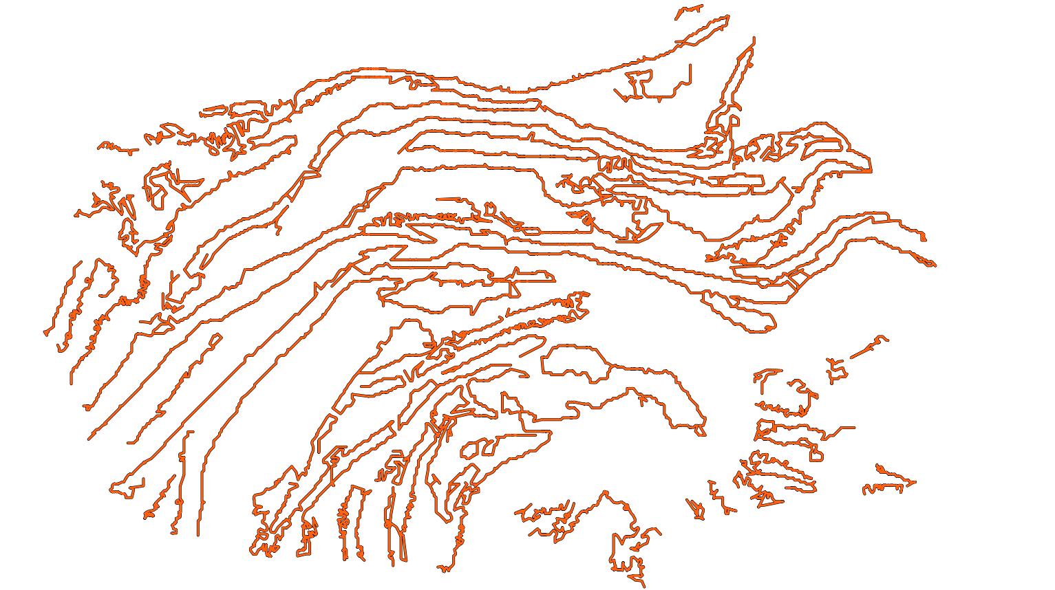
Figure representing the extracted curves. — Visualization of the extracted cruves representing breaklines.

Post-processing

Once clusters are available, it might be useful to apply some post-processing to derive useful information from them. That is what post-processing components aim to do. They can be defined in the "post_clustering" list. The execution will start by the first component in the list and will end at the last one, i.e., it is sequential with respect to the order in the list.

ClusterEnveloper

The ClusterEnveloper can be used to find the geometry enclosing the points. Envelopes often support the estimation of the enclosed volume. They can be exported to output files. The JSON below shows how to define a cluster enveloper post-processor inside the post-processing pipeline of a clusterer.

"post_clustering": [
    {
        "post-processor": "ClusterEnveloper",
        "envelopes": [
            {
                "type": "AlignedBoundingBox",
                "compute_volume": true,
                "output_path": "*/aabbs.csv",
                "separator": ","
            },
            {
                "type": "BoundingBox",
                "compute_volume": true,
                "output_path": "*/bboxes.csv",
                "separator": ","
            }
        ]
    }
]

The JSON above defines a ClusterEnveloper that will compute the axis-aligned bounding box and also the oriented bounding box. The volume will be computed for each envelope and they will be exported to a CSV file. More concretely, each row in the CSV will contain three coordinates representing a vertex, an integer representing the cluster label, and the estimated volume. All the values will be separated by ,.

Arguments

– envelopes

List of envelopes that must be computed by the ClusterEnveloper

– type

The type of the envelope, it can be "AxisAlignedBoundingBox" or "BoundingBox" (the edges of the last one are not necessarily parallel to the vectors of the canonical basis).

– compute_volume

Flag to specify whether to compute the volume enclosed by the envelope (true) or not (false).

– output_path

The path where the envelope’s data will be exported (typically in CSV format).

– separator

The separator to be used in the output CSV file.

ClusterMarker

The ClusterMarker can be used to compute a point for each cluster to represent it. These points can be exported as CSV files or shapefiles. The JSON below shows how to define a cluster marker post-processor inside the post-processing pipeline of a clusterer.

"post_clustering": [
    {
        "post-processor": "ClusterMarker",
        "strategy": "centroid",
        "proj_str": null,
        "epsg": 32630,
        "output_path": "*/marks.shp",
        "nthreads": -1
    }
]

The JSON above defines a ClusterMarker that will compute the centroid for each cluster as a marker. The output will be exported in the EPSG:32630 CRS to a shapefile called marks.shp. The computations will be carried out using all the cores available in the system.

Arguments

– strategy: The strategy that must be used to compute the markers. Supported strategies are "centroid", (see ClusterMarker.compute_cluster_centroid()), "midrange" (see ClusterMarker.compute_cluster_midrange()), "medianoid" (see ClusterMarker.compute_cluster_medianoid()), "medoid" (see ClusterMarker.compute_cluster_medoid()), and "geometric_median" (see ClusterMarker.compute_cluster_geometric_median()).
– proj_str: The coordinate reference system specified as a projection string (proj).
– epsg: Can be optionally used to specified the CRS following the European Petroleum Survey Groups (EPSG) standard format.
– nthreads: The number of threads that must be used for the parallel computations. Note that -1 means using as many threads as available cores.
– output_path: The output path where the markers must be written. Note that if the extension is .shp, then the output will be written as a shapefile. Otherwise, it will be written as an ASCII CSV file.

ClusterSelector

The ClusterSelector can be used to discard those clusters that do not satisfy satisfy some given criteria. It consists of a list of filters that check some given relationals and either preserve or discard those clusters that satisfy them. The JSON below shows how to define a cluster enveloper post-processor inside the post-processing pipeline of a clusterer.

"post_clustering": [
    {
        "post-processor": "ClusterSelector",
        "filters": [
          {
            "attribute": "number_of_points",
            "relational": "greater_than_or_equal_to",
            "target": 256,
            "action": "preserve"
          },
          {
            "attribute": "surface_area",
            "relational": "less_than",
            "target": 1,
            "action": "discard"
          },
          {
            "attribute": "z_length",
            "relational": "less_than",
            "target": 3,
            "action": "discard"
          }
        ]
    }
]

The JSON above defines a ClusterSelector that will preserve only the clusters with at least \(256\) points and discard those whose convex hull has a surface area less than \(1\) meter or whose length along the \(z\)-axis is below the \(3\) meters.

Arguments

– filters

The list of filters based on relational conditions to decide whether to preserve or discard those clusters who satisfy them.

– attribute: The attribute involved in the relational condition as the left-hand side. Supported attributes are "number_of_points", "surface_area", "volume", "surface_density", "volume_density", "x_length", "y_length" and "z_length". Their description can be read in the documentation of ClusterSelector.
– relational: The relational governing the condition. Supported relationals are "not_equals" \(x \neq y\), "equals" \(x = y\), "less_than" \(x < y\), "less_than_or_equal_to" \(x \leq y\), "greater_than" \(x > y\), "greater_than_or_equal_to" \(x \geq y\), "in" \(x \in S\), "not_in" \(x \notin S\), and "inside" \(x \in [a, b] \subset \mathbb{R}\).
– target: The right-hand side of the relational condition.
– action: Whether to "preserve" or "discard" the clusters that satisfy the relational condition.

Decorators

Furthest point sampling decorator

The FPSDecoratorTransformer can be used to decorate a data clusterer such that the computations can take place in a transformed space of reduced dimensionality. Typically, the domain of a clustering is the entire point cloud, let us say \(m\) points. When using a FPSDecoratedClusterer this domain will be transformed to a subset of the original point cloud with \(R\) points, such that \(m \geq R\). Decorating a clusterer with this decorator can be useful to reduce its execution time.

{
    "clustering": "fpsdecorated",
    "fps_decorator": {
        "num_points": "m/10",
        "fast": true,
        "num_encoding_neighbors": 1,
        "num_decoding_neighbors": 1,
        "release_encoding_neighborhoods": false,
        "threads": 16,
        "representation_report_path": null
    },
    "decorated_clusterer": {
        "clustering": "dbscan",
        "cluster_name": "cluster_wood",
        "precluster_name": "prediction",
        "precluster_domain": [1],
        "min_points": 200,
        "radius": 3.0,
        "post_clustering": [
            {
                "post-processor": "ClusterEnveloper",
                "envelopes": [
                    {
                        "type": "AlignedBoundingBox",
                        "compute_volume": true,
                        "output_path": "*/aabbs.csv",
                        "separator": ","
                    },
                    {
                        "type": "BoundingBox",
                        "compute_volume": true,
                        "output_path": "*/bboxes.csv",
                        "separator": ","
                    }
                ]
            }
        ]
    }
}

Arguments

– fps_decorator

The specification of the furthest point sampling (FPS) decoration carried out through the FPSDecoratorTransformer.

– num_points: The target number of points \(R\) for the transformed point cloud. It can be an integer or an expression that will be evaluated with \(m\) representing the number of points of the original point cloud, e.g., "m/2" will downscale the point cloud to half the number of points.
– fast: Whether to use exact furthest point sampling (false) or a faster stochastic approximation (true).
– num_encoding_neighbors: How many closest neighbors in the original point cloud are considered for each point in the transformed point cloud to reduce from the original space to the transformed one.
– num_decoding_neighbors: How many closest neighbors in the transformed point cloud are considered for each point in the original point cloud to propagate back from the transformed space to the original one.
– release_encoding_neighborhoods: Whether the encoding neighborhoods can be released after computing the transformation (true) or not (false). Releasing these neighborhoods means the FPSDecoratorTransformer.reduce() method must not be called, otherwise errors will arise. Setting this flag to true can help saving memory when needed.
– threads: The number of parallel threads to consider for the parallel computations. Note that -1 means using as many threads as available cores.
– representation_report_path: Where to export the transformed point cloud. In general, it should be null to prevent unnecessary operations. However, it can be enabled (by given any valid path to write a point cloud file) to visualize the points that are seen by the data miner.

– decorated_clusterer

A typical clustering specification. See the DBScan clusterer for an example.

Minimum distance decimator decorator

The MinDistDecimatorDecorator can be used to decorate a clusterer such that the computations can take place in a transformed space of reduced dimensionality. Typically, the domain of a clusterer is the entire point cloud, let us say \(m\) points. When using a MinDistDecoratedClusterer this domain will be transformed to a subset of the original point cloud with \(R \leq m\) points. This representation is achieved by assuring that no point is closer to its closest neighbor than a given minimum distance threshold. Decorating a clusterer with this decorator can be useful to reduce its execution time.

{
    "clustering": "MinDistDecorated",
    "mindist_decorator": {
        "min_distance": 0.3,
        "num_encoding_neighbors": 1,
        "num_decoding_neighbors": 1,
        "release_encoding_neighborhoods": false,
        "threads": -1,
        "representation_report_path": null
    },
    "decorated_clusterer": {
        "clustering": "dbscan",
        "cluster_name": "bunny",
        "precluster_name": "classification",
        "min_points": 3,
        "radius": 3.0
    }
}

Arguments

– mindist_decorator: See the minimum distance decorated miner documentation about arguments .
– decorated_clusterer: A typical clustering specification. See the DBScan clusterer for an example.