Deep learning

Deep learning models can be seen as a subset of machine learning models, typically based on artificial neural networks. Using deep learning models for point cloud processing often demands top-level hardware. Users interested in these models are strongly encouraged to have a computer with no less than \(128\,\mathrm{GB}\) of RAM, a manycore processor (with many real cores for efficient parallel processing), and a top-level coprocessor like a GPU or a TPU. It is worth mentioning that training deep learning models for dense point clouds is not feasible with a typical CPU, so the coprocessor is a must. However, using an already trained deep learning model might be possible without a coprocessor, provided the system has a top-level CPU and high amounts of RAM.

The deep learning models in the VL3D framework are based on the strategy represented in the figure below. First, it is necessary to select a set of neighborhoods that represents the input point cloud. These can overlap between themselves, i.e., the same point can be in more than one neighborhood. The neighborhoods can be defined as spheres, voxels, cylinders, or many more. Now, note that each neighborhood can contain a different number of points. In the VL3D framework, the input neighborhoods must be transformed into fixed-size representations (in terms of the number of points) that will be later grouped into batches to be fed into the neural network.

Once the neural network has computed the output, it will be propagated back from the fixed-size receptive fields to the original neighborhoods, for example, through a nearest-neighbor strategy. As there might be many outputs for the same point, the values in the neighborhoods are aggregated (also reduced), so there is one final value per point in the original point cloud (provided that the input neighborhoods cover the entire point cloud).

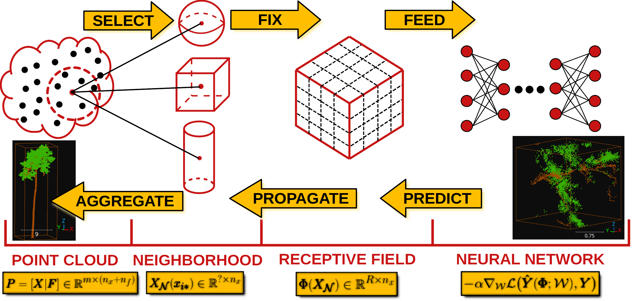
Visualization of the deep learning strategy used by the VL3D framework.

The VL3D framework uses Keras and TensorFlow as the deep learning backend. The usage of deep learning models is documented below. However, for this documentation users are expected to be already familiar with the framework, especially with how to define pipelines. If that is not the case, we strongly encourage you to read the documentation about pipelines before.

Models

PointNet-based point-wise classifier

The PointNetPwiseClassif can be used to solve point-wise classification tasks. This model is based on the PointNet architecture and it can be defined as shown in the JSON below:

{
    "train": "PointNetPwiseClassifier",
    "fnames": ["AUTO"],
    "training_type": "base",
    "random_seed": null,
    "model_args": {
        "num_classes": 5,
        "class_names": ["Ground", "Vegetation", "Building", "Urban furniture", "Vehicle"],
        "num_pwise_feats": 16,
        "pre_processing": {
            "pre_processor": "furthest_point_subsampling",
            "to_unit_sphere": false,
            "support_strategy": "grid",
            "support_chunk_size": 2000,
            "support_strategy_fast": false,
            "_training_class_distribution": [1000, 1000, 1000, 1000, 1000],
            "center_on_pcloud": true,
            "num_points": 4096,
            "num_encoding_neighbors": 1,
            "fast": false,
            "neighborhood": {
                "type": "rectangular3D",
                "radius": 5.0,
                "separation_factor": 0.8
            },
            "nthreads": 12,
            "training_receptive_fields_distribution_report_path": "*/training_eval/training_receptive_fields_distribution.log",
            "training_receptive_fields_distribution_plot_path": "*/training_eval/training_receptive_fields_distribution.svg",
            "training_receptive_fields_dir": "*/training_eval/training_receptive_fields/",
            "receptive_fields_distribution_report_path": "*/training_eval/receptive_fields_distribution.log",
            "receptive_fields_distribution_plot_path": "*/training_eval/receptive_fields_distribution.svg",
            "receptive_fields_dir": "*/training_eval/receptive_fields/",
            "training_support_points_report_path": "*/training_eval/training_support_points.las",
            "support_points_report_path": "*/training_eval/support_points.las"
        },
        "kernel_initializer": "he_normal",
        "pretransf_feats_spec": [
            {
                "filters": 32,
                "name": "prefeats32_A"
            },
            {
                "filters": 32,
                "name": "prefeats_32B"
            },
            {
                "filters": 64,
                "name": "prefeats_64"
            },
            {
                "filters": 128,
                "name": "prefeats_128"
            }
        ],
        "postransf_feats_spec": [
            {
                "filters": 128,
                "name": "posfeats_128"
            },
            {
                "filters": 256,
                "name": "posfeats_256"
            },
            {
                "filters": 64,
                "name": "posfeats_end_64"
            }
        ],
        "tnet_pre_filters_spec": [32, 64, 128],
        "tnet_post_filters_spec": [128, 64, 32],
        "final_shared_mlps": [512, 256, 128],
        "skip_link_features_X": false,
        "include_pretransf_feats_X": false,
        "include_transf_feats_X": true,
        "include_postransf_feats_X": false,
        "include_global_feats_X": true,
        "skip_link_features_F": false,
        "include_pretransf_feats_F": false,
        "include_transf_feats_F": true,
        "include_postransf_feats_F": false,
        "include_global_feats_F": true,
        "model_handling": {
            "summary_report_path": "*/model_summary.log",
            "training_history_dir": "*/training_eval/history",
            "class_weight": [0.25, 0.5, 0.5, 1, 1],
            "training_epochs": 200,
            "batch_size": 16,
            "checkpoint_path": "*/checkpoint.weights.h5",
            "checkpoint_monitor": "loss",
            "learning_rate_on_plateau": {
                "monitor": "loss",
                "mode": "min",
                "factor": 0.1,
                "patience": 2000,
                "cooldown": 5,
                "min_delta": 0.01,
                "min_lr": 1e-6
            },
            "early_stopping": {
                "monitor": "loss",
                "mode": "min",
                "min_delta": 0.01,
                "patience": 5000
            },
            "prediction_reducer": {
                "reduce_strategy" : {
                    "type": "MeanPredReduceStrategy"
                },
                "select_strategy": {
                    "type": "ArgMaxPredSelectStrategy"
                }
            }
        },
        "compilation_args": {
            "optimizer": {
                "algorithm": "SGD",
                "learning_rate": {
                    "schedule": "exponential_decay",
                    "schedule_args": {
                        "initial_learning_rate": 1e-2,
                        "decay_steps": 2000,
                        "decay_rate": 0.96,
                        "staircase": false
                    }
                }
            },
            "loss": {
                "function": "class_weighted_categorical_crossentropy"
            },
            "metrics": [
                "categorical_accuracy"
            ]
        },
        "architecture_graph_path": "*/model_graph.png",
        "architecture_graph_args": {
            "show_shapes": true,
            "show_dtype": true,
            "show_layer_names": true,
            "rankdir": "TB",
            "expand_nested": true,
            "dpi": 300,
            "show_layer_activations": true
        }
    },
    "training_evaluation_metrics": ["OA", "P", "R", "F1", "IoU", "wP", "wR", "wF1", "wIoU", "MCC", "Kappa"],
    "training_class_evaluation_metrics": ["P", "R", "F1", "IoU"],
    "training_evaluation_report_path": "*/training_eval/evaluation.log",
    "training_class_evaluation_report_path": "*/training_eval/class_evaluation.log",
    "training_confusion_matrix_report_path": "*/training_eval/confusion.log",
    "training_confusion_matrix_plot_path": "*/training_eval/confusion.svg",
    "training_class_distribution_report_path": "*/training_eval/class_distribution.log",
    "training_class_distribution_plot_path": "*/training_eval/class_distribution.svg",
    "training_classified_point_cloud_path": "*/training_eval/classified_point_cloud.las",
    "training_activations_path": "*/training_eval/activations.las"
}

The JSON above defines a PointNetPwiseClassif that uses a furthest point subsampling strategy with a 3D rectangular neighborhood. The optimization algorithm to train the neural network is stochastic gradient descent (SGD). The loss function is a categorical cross-entropy that accounts for class weights. The class weights can be used to handle data imbalance.

Arguments

– fnames

The names of the features that must be considered by the neural network.

– training_type

Typically it should be "base" for neural networks. For further details, read the training strategies section.

– random_seed

Can be used to specify an integer like seed for any randomness-based computation. Mostly to be used for reproducibility purposes. Note that the initialization of a neural network is often based on random distributions. This parameter does not affect those distributions, so it will not guarantee reproducibility for of deep learning models.

– model_args

The model specification.

– fnames

If the input to the model involves features, their names must be given again inside the model_args dictionary due to technical reasons.

– num_classess

An integer specifying the number of classes involved in the point-wise classification tasks.

– class_names

The names of the classes involved in the classification task. Each string corresponds to the class associated to its index in the list.

– num_pwise_feats

How many point-wise features must be computed.

– pre_processing

How the select and fix stages of the deep learning strategy must be handled. See the receptive fields section for further details.

– kernel_initializer

The name of the kernel initialization method. See Keras documentation on layer initializers for further details.

– pretransf_feats_spec

A list of dictionaries where each dictionary defines a layer to be placed before the transformation block in the middle. Each dictionary must contain filters (an integer specifying the output dimensionality of the layer) and name (a string representing the layer’s name).

– postransf_feats_spec

A list of dictionaries where each dictionary defines a layer to be placed after the transformation block in the middle. Each dictionary must contain filters (an integer specifying the output dimensionality of the layer) and name (a string representing the layer’s name).

– tnet_pre_filters_spec

A list of integers where each integer specifies the output dimensionality of a convolutional layer placed before the global pooling.

– tnet_post_filters_spec

A list of integers where each integer specifies the output dimensionality of a dense layer (MLP) placed after the global pooling.

– final_shared_mlps

A list of integers where each integer specifies the output dimensionality of the shared MLP (i.e., 1D Conv with unitary window and stride). These are called final because they are applied immediately before the convolution that reduces the number of point-wise features that constitute the input of the final layer.

– skip_link_features_X

Whether to propagate the input structure space to the final concatenation of features (True) or not (False).

– include_pretransf_feats_X

Whether to propagate the values of the hidden layers that processed the structure space before the second transformation block to the final concatenation of features (True) or not (False).

– include_transf_feats_X

Whether to propagate the values of the hidden layers that processed the structure space in the second transformation block to the final concatenation of features (True) or not (False).

– include_postransf_feats_X

Whether to propagate the values of the hidden layers that processed the structure space after the second transformation block to the final concatenation of features (True) or not (False).

– include_global_feats_X

Whether to propagate the global features derived from the structure space to the final concatenation of features (True) or not (False).

– skip_link_features_F

Whether to propagate the input feature space to the final concatenation of features (True) or not (False).

– include_pretransf_feats_F

Whether to propagate the values of the hidden layers that processed the feature space before the second transformation block to the final concatenation of features (True) or not (False).

– include_transf_feats_F

Whether to propagate the values of the hidden layers that processed the feature space in the second transformation block to the final concatenation of features (True) or not (False).

– include_postransf_feats_F

Whether to propagate the values of the hidden layers that processed the feature space after the second transformation block to the final concatenation of features (True) or not (False).

– include_global_feats_F

Whether to propagate the global features derived from the feature space to the final concatenation of features (True) or not (False).

– features_structuring_layer EXPERIMENTAL

Specification for the FeaturesStructuringLayer that uses radial basis functions to transform the features. This layer is experimental and it is not part of typical PointNet-like architectures. Users are strongly encouraged to avoid using this layer. At the moment it is experimental and should only be used for development and research purposes.

– architecture_graph_path

Path where the plot representing the neural network’s architecture wil be exported.

– architecture_graph_args

Arguments governing the architecture’s graph. See Keras documentation on plot_model for further details.

– model_handling

Define how to handle the model, i.e., not the architecture itself but how it must be used.

– summary_report_path

Path where a text describing the built network’s architecture must be exported.

– training_history_dir

Path where the data (plots and text) describing the training process must be exported.

– class_weight

The class weights for the model’s loss. It can be null in which case no class weights will be considered. Alternatively, it can be "AUTO" to automatically compute the class weights based on TensorFlow’s imbalanced data tutorial. It can also be a list with as many elements as classes where each element governs the class weight for the corresponding class.

– focusing_parameter

The focusing parameter governing focal loss functions. By default, it is \(\gamma=2\). Note that non-focal losses will simply ignore this parameter.

– training_epochs

How many epochs must be considered to train the model.

– batch_size

How many receptive fields per batch must be grouped together as input for the neural network.

– checkpoint_path

Path where a checkpoint of the model’s current status can be exported. When given, it will be used during training to keep the best model. The extension of the file must be necessarily ".weights.h5".

– checkpoint_monitor

What metric must be analyzed to decide what is the best model when using the checkpoint strategy. See the Keras documentation on ModelCheckpoint for more information.

– learning_rate_on_plateau

When given, it can be used to configure the learning rate on plateau callback. See the Keras documentation on ReduceLROnPlateau for more information.

– early_stopping

When given, it can be used to configure the early stopping callback. See the Keras documentation on EarlyStopping for more information.

– prediction_reducer

Can be used to modify the default prediction reduction strategies. It is a dictionary that supports a "reduce_strategy" specification and also a "select_strategy" specification.

– reduce_strategy

Supported types are SumPredReduceStrategy, MeanPredReduceStrategy (default), MaxPredReduceStrategy, and EntropicPredReduceStrategy.

– select_strategy

Supported types are ArgMaxPredSelectStrategy (default).

– fit_verbose

Whether to use silent mode (0), show a progress bar (1), or print one line per epoch (2) when training a model. Alternatively, "auto" can be used, which typically means (1).

– predict_verbose

Whether to use silent mode (0), show a progress bar (1), or print one line per epoch (2) when using a model to predict. Alternatively, "auto" can be used, which typically means (1).

– compilation_args

The arguments governing the model’s compilation. They include the optimizer, the loss function and the metrics to be monitored during training. See the optimizers section and losses section for further details.

– training_evaluation_metrics

What metrics must be considered to evaluate the model on the training data.

• "OA" Overall accuracy.

• "P" Precision.

• "R" Recall.

• "F1" F1 score (harmonic mean of precision and recall).

• "IoU" Intersection over union (also known as Jaccard index).

• "wP" Weighted precision (weights by the number of true instances for each class).

• "wR" Weighted recall (weights by the number of true instances for each class).

• "wF1" Weighted F1 score (weights by the number of true instances for each class).

• "wIoU" Weighted intersection over union (weights by the number of true instances for each class).

• "MCC" Matthews correlation coefficient.

• "Kappa" Cohen’s kappa score.

– training_class_evaluation_metrics

What class-wose metrics must be considered to evaluate the model on the training data.

• "P" Precision.

• "R" Recall.

• "F1" F1 score (harmonic mean of precision and recall).

• "IoU" Intersection over union (also known as Jaccard index).

– training_evaluation_report_path

Path where the report about the model evaluated on the training data must be exported.

– training_class_evaluation_report_path

Path where the report about the model’s class-wise evaluation on the training data must be exported.

– training_confusion_matrix_report_path

Path where the confusion matrix must be exported (in text format).

– training_confusion_matrix_plot_path

Path where the confusion matrix must be exported (in image format).

– training_class_distribution_report_path

Path where the analysis of the classes distribution must be exported (in text format).

– training_class_distribution_plot_path

Path where the analysis of the classes distribution must be exported (in image format).

– training_classifier_point_cloud_path

Path where the training data with the model’s predictions must be exported.

– training_activations_path

Path where a point cloud representing the point-wise activations of the model must be exported. It might demand a lot of memory. However, it can be useful to understand, debug, and improve the model.

Hierarchical autoencoder point-wise classifier

Hierarchical autoencoders for point-wise classification are available in the framework through the ConvAutoencPwiseClassif architecture. They are also referred to in the documentation as convolutional autoencoders. In the scientific literature they are widely known as hierarchical feature extractors too. The figure below summarized the main logic of hierarchical autoencoders for point clouds.

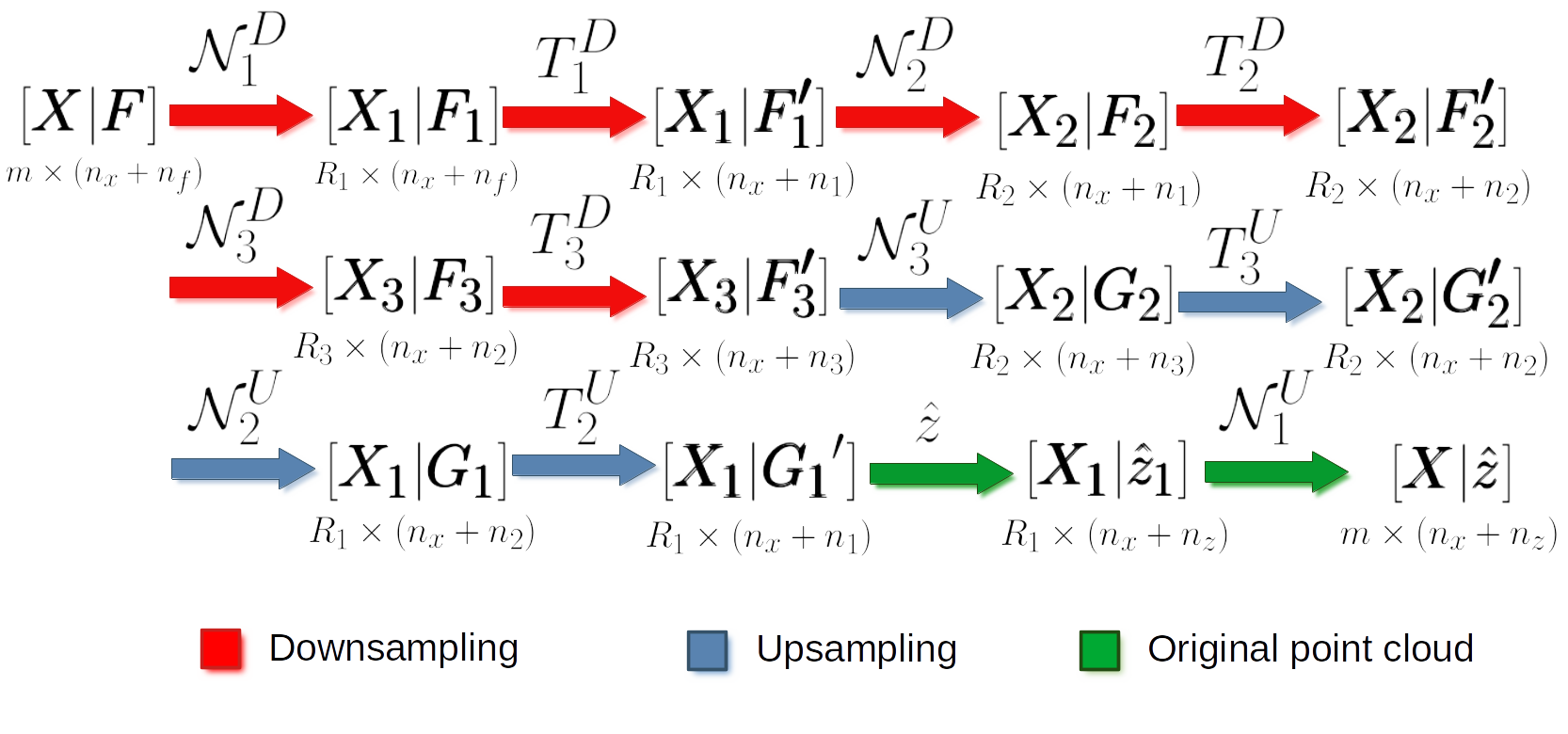
Representation of the main logic governing hierarchical autoencoders for point clouds based on hierarchical receptive fields.

Initially, we have a 3D structure space \(\pmb{X} \in \mathbb{R}^{m \times 3}\) with \(m\) points and the corresponding feature space \(\pmb{F} \in \mathbb{R}^{m \times n_f}\) with \(n_f\) features. For a given depth, for example for depth three (as illustrated in the figure above), there is a set of downsampling stages followed by a set of upsampling stages.

At a given depth \(d\), there is a non downsampled structure space \(\pmb{X_{d-1}} \in \mathbb{R}^{R_{d-1} \times 3}\) and its corresponding \(\pmb{X_{d}} \in \mathbb{R}^{R_d \times 3}\) downsampled version. The neighborhood \(\mathcal{N}_d^D\) can be represented with an indexing matrix \(\pmb{N}_{d}^{D} \in \mathbb{Z}^{R_d \times \kappa_d^D}\) that defines for each of the \(R_d\) points in the downsampled space its \(\kappa_d^D\) closest neighbors in the non downsampled space.

Once in the downsampling space, a transformation \(T_d^D\) is applied to downsampled feature space to obtain a new set of features. This transformation can be done using different operators like PointNet or Kernel Point Convolution (KPConv). Further details about them will be given below in the hierarchical feature extraction with PointNet and the hierarchical feature extraction with KPConv sections.

After finishing the downsampling and feature extraction operations, it is time to restore the original dimensionality through upsampling. First, the \(\mathcal{N}_d^U\) neighborhood is reresented by an indexing matrix \(\pmb{N}_{d}^U \in \mathbb{Z}^{R_{d-1} \times \kappa_d^U}\) that defines for each of the \(R_{d-1}\) points in the upsampled space its \(\kappa_d^U\) closest neighbors in the non upsampled space. Then, the \(T_d^U\) upsampling operation is applied. Typically, it is a SharedMLP (i.e., a unitary 1D discrete convolution).

Note that the last upsampling operation is not applied inside the neural network. Instead, the estimations of the network are computed on the first receptive field with structure space \(\pmb{X_1} \in \mathbb{R}^{R_1 \times 3}\) (the one with more points, and thus, closer to the original neighborhood). Finally, the last upsampling is computed to transform the predictions of the neural network (\(\hat{z}\)) back to the original input neighborhood (with an arbitrary number of points).

Hierarchical feature extraction with PointNet

The ConvAutoencPwiseClassif architecture can be configured with PointNet for feature extraction operations. The downsampling strategy can be defined through the FeaturesDownsamplingLayer, the upsampling strategy through the FeaturesUpsamplingLayer, and the feature extraction through the GroupingPointNetLayer. The JSON below illustrates how to configure PointNet++-like hierarchical feature extractors using the VL3D framework. For further details on the original PointNet++ architecture, readers are referred to the PointNet++ paper (Qi et al., 2017) .

{
  "in_pcloud": [
    "/mnt/netapp2/Store_uscciaep/lidar_data/hessigheim/data/Mar18_train.laz"
  ],
  "out_pcloud": [
    "/mnt/netapp2/Store_uscciaep/lidar_data/hessigheim/vl3d/hae_X_FPS50K/T1/*"
  ],
  "sequential_pipeline": [
    {
        "train": "ConvolutionalAutoencoderPwiseClassifier",
        "training_type": "base",
        "fnames": ["AUTO"],
        "random_seed": null,
        "model_args": {
            "num_classes": 11,
            "class_names": ["LowVeg", "ImpSurf", "Vehicle", "UrbanFurni", "Roof", "Facade", "Shrub", "Tree", "Soil/Gravel", "VertSurf", "Chimney"],
            "pre_processing": {
                "pre_processor": "hierarchical_fps",
                "support_strategy_num_points": 50000,
                "to_unit_sphere": false,
                "support_strategy": "fps",
                "support_chunk_size": 2000,
                "support_strategy_fast": true,
                "center_on_pcloud": true,
                "neighborhood": {
                    "type": "rectangular3D",
                    "radius": 3.0,
                    "separation_factor": 0.8
                },
                "num_points_per_depth": [512, 256, 128, 64, 32],
                "fast_flag_per_depth": [false, false, false, false, false],
                "num_downsampling_neighbors": [1, 16, 8, 8, 4],
                "num_pwise_neighbors": [32, 16, 16, 8, 4],
                "num_upsampling_neighbors": [1, 16, 8, 8, 4],
                "nthreads": 12,
                "training_receptive_fields_distribution_report_path": "*/training_eval/training_receptive_fields_distribution.log",
                "training_receptive_fields_distribution_plot_path": "*/training_eval/training_receptive_fields_distribution.svg",
                "training_receptive_fields_dir": null,
                "receptive_fields_distribution_report_path": "*/training_eval/receptive_fields_distribution.log",
                "receptive_fields_distribution_plot_path": "*/training_eval/receptive_fields_distribution.svg",
                "receptive_fields_dir": null,
                "training_support_points_report_path": "*/training_eval/training_support_points.las",
                "support_points_report_path": "*/training_eval/support_points.las"
            },
            "feature_extraction": {
                "type": "PointNet",
                "operations_per_depth": [2, 1, 1, 1, 1],
                "feature_space_dims": [64, 64, 128, 256, 512, 1024],
                "bn": true,
                "bn_momentum": 0.0,
                "H_activation": ["relu", "relu", "relu", "relu", "relu", "relu"],
                "H_initializer": ["glorot_uniform", "glorot_uniform", "glorot_uniform", "glorot_uniform", "glorot_uniform", "glorot_uniform"],
                "H_regularizer": [null, null, null, null, null, null],
                "H_constraint": [null, null, null, null, null, null],
                "gamma_activation": ["relu", "relu", "relu", "relu", "relu", "relu"],
                "gamma_kernel_initializer": ["glorot_uniform", "glorot_uniform", "glorot_uniform", "glorot_uniform", "glorot_uniform", "glorot_uniform"],
                "gamma_kernel_regularizer": [null, null, null, null, null, null],
                "gamma_kernel_constraint": [null, null, null, null, null, null],
                "gamma_bias_enabled": [true, true, true, true, true, true],
                "gamma_bias_initializer": ["zeros", "zeros", "zeros", "zeros", "zeros", "zeros"],
                "gamma_bias_regularizer": [null, null, null, null, null, null],
                "gamma_bias_constraint": [null, null, null, null, null, null]
            },
            "_structure_alignment": {
                "tnet_pre_filters_spec": [64, 128, 256],
                "tnet_post_filters_spec": [128, 64, 32],
                "kernel_initializer": "glorot_normal"
            },
            "features_alignment": null,
            "downsampling_filter": "gaussian",
            "upsampling_filter": "mean",
            "upsampling_bn": true,
            "upsampling_momentum": 0.0,
            "conv1d_kernel_initializer": "glorot_normal",
            "output_kernel_initializer": "glorot_normal",
            "model_handling": {
                "summary_report_path": "*/model_summary.log",
                "training_history_dir": "*/training_eval/history",
                "features_structuring_representation_dir": "*/training_eval/feat_struct_layer/",
                "class_weight": [1, 1, 1, 1, 1, 1, 1, 1, 1, 1, 1],
                "training_epochs": 200,
                "batch_size": 16,
                "checkpoint_path": "*/checkpoint.weights.h5",
                "checkpoint_monitor": "loss",
                "learning_rate_on_plateau": {
                    "monitor": "loss",
                    "mode": "min",
                    "factor": 0.1,
                    "patience": 2000,
                    "cooldown": 5,
                    "min_delta": 0.01,
                    "min_lr": 1e-6
                }
            },
            "compilation_args": {
                "optimizer": {
                    "algorithm": "SGD",
                    "learning_rate": {
                        "schedule": "exponential_decay",
                        "schedule_args": {
                            "initial_learning_rate": 1e-2,
                            "decay_steps": 15000,
                            "decay_rate": 0.96,
                            "staircase": false
                        }
                    }
                },
                "loss": {
                    "function": "class_weighted_categorical_crossentropy"
                },
                "metrics": [
                    "categorical_accuracy"
                ]
            },
            "architecture_graph_path": "*/model_graph.png",
            "architecture_graph_args": {
                "show_shapes": true,
                "show_dtype": true,
                "show_layer_names": true,
                "rankdir": "TB",
                "expand_nested": true,
                "dpi": 300,
                "show_layer_activations": true
            }
        },
        "autoval_metrics": ["OA", "P", "R", "F1", "IoU", "wP", "wR", "wF1", "wIoU", "MCC", "Kappa"],
        "training_evaluation_metrics": ["OA", "P", "R", "F1", "IoU", "wP", "wR", "wF1", "wIoU", "MCC", "Kappa"],
        "training_class_evaluation_metrics": ["P", "R", "F1", "IoU"],
        "training_evaluation_report_path": "*/training_eval/evaluation.log",
        "training_class_evaluation_report_path": "*/training_eval/class_evaluation.log",
        "training_confusion_matrix_report_path": "*/training_eval/confusion.log",
        "training_confusion_matrix_plot_path": "*/training_eval/confusion.svg",
        "training_class_distribution_report_path": "*/training_eval/class_distribution.log",
        "training_class_distribution_plot_path": "*/training_eval/class_distribution.svg",
        "training_classified_point_cloud_path": "*/training_eval/classified_point_cloud.las",
        "training_activations_path": null
    },
    {
      "writer": "PredictivePipelineWriter",
      "out_pipeline": "*pipe/HAE_T1.pipe",
      "include_writer": false,
      "include_imputer": false,
      "include_feature_transformer": false,
      "include_miner": false,
      "include_class_transformer": false
    }
  ]
}

The JSON above defines a ConvAutoencPwiseClassif that uses a hierarchical furthest point sampling strategy with a 3D rectangular neighborhood and the PointNet operator for feature extraction. It is expected to work only on the structure space, i.e., the input feature space will be a single column of ones.

Arguments

– training_type

Typically it should be "base" for neural networks. For further details, read the training strategies section.

– fnames

The name of the features that must be given as input to the neural network. For hierarchical autoencoders this list can contain "ones" to specify whether to include a column of ones in the input space matrix. This architecture does not support empty feature spaces as input, thus, when no features are given, the input feature space must be represented with a column of ones.

– random_seed

Can be used to specify an integer like seed for any randomness-based computation. Mostly to be used for reproducibility purposes. Note that the initialization of a neural network is often based on random distributions. This parameter does not affect those distributions, so it will not guarantee reproducibility for of deep learning models.

– model_args

The model specification.

– num_classess

An integer specifying the number of classes involved in the point-wise classification tasks.

– class_names

The names of the classes involved in the classification task. Each string corresponds to the class associated to its index in the list.

– pre_processing

How the select and fix stages of the deep learning strategy must be handled. Note that hierarchical autoencoders demand hierarchical receptive fields. See the receptive fields and hierarchical FPS receptive field sections for further details.

– feature_extraction

The definition of the feature extraction operator. A detailed description of the case when "type": "PointNet" is given below. For a description of the case when "type": "KPConv" see the KPConv operator documentation.

– operations_per_depth

A list specifying how many operations per depth level. The i-th element of the list gives the number of feature extraction operations at depth i.

– feature_space_dims

A list specifying the output dimensionality of the feature space after each feature extraction operation. The i-th element of the list gives the dimensionality of the i-th feature extraction operation.

– bn

Boolean flag to decide whether to enable batch normalization for feature extraction.

– bn_momentum

Momentum for the moving average of the batch normalization, such that new_mean = old_mean * momentum + batch_mean * (1 - momentum). See the Keras documentation on batch normalization for more details.

– H_activation

The activation function for the SharedMLP of each feature extraction operation. See the keras documentation on activations for more details.

– H_initializer

The initialization method for the SharedMLP of each feature extraction operation. See the keras documentation on initializers for more details.

– H_regularizer

The regularization strategy for the SharedMLP of each feature extraction operation. See the keras documentation on regularizers for more details.

– H_constraint

The constraints for the SharedMLP of each feature extraction operation. See the keras documentation on constraints for more details.

– gamma_activation

The constraints for the MLP of each feature extraction operation. See the keras documentation on activations for more details.

– gamma_kernel_initializer

The initialization method for the MLP of each feature extraction operation (ignoring the bias term). See the keras documentation on initializers for more details.

– gamma_kernel_regularizer

The regularization strategy for the MLP of each feature extraction operation (ignoring the bias term). See the keras documentation on regularizers for more details.

– gamma_kernel_constraint

The constraints for the MLP of each feature extraction operation (ignoring the bias term). See the keras documentation on constraints for more details.

– gamma_bias_enabled

Whether to enable the bias term for the MLP of each feature extraction operation.

– gamma_bias_initializer

The initialization method for the bias term of the MLP of each feature extraction operation. See the keras documentation on initializers for more details.

– gamma_bias_regularizer

The regularization strategy for the bias term of the MLP of each feature extraction operation. See the keras documentation on regularizers for more details.

– gamma_bias_constraint

The constraints for the bias term of the MLP of each feature extraction operation. See the keras documentation on constraints for more details.

– structure_alignment

When given, this specification will govern the alignment of the structure space.

– tnet_pre_filters_spec

List defining the number of pre-transformation filters at each depth.

– tnet_post_filters_spec

List defining the number of post-transformation filters at each depth.

– kernel_initializer

The kernel initialization method for the structure alignment layers. See the keras documentation on initializers for more details.

– features_alignment

When given, this specification will govern the alignment of the feature space. It is like the structure_alignment dictionary but it is applied to the features instead of the structure space. It must be null to mimic a classical KPConv model.

– downsampling_filter

The type of downsampling filter. See FeaturesDownsamplingLayer, StridedKPConvLayer, StridedLightKPConvLayer, and InterdimensionalPointTransformerLayer for more details.

– upsampling_filter

The type of upsampling filter. See FeaturesUpsamplingLayer and InterdimnsionalPointTransformerLayer for more details.

– upsampling_bn

Boolean flag to decide whether to enable batch normalization for upsampling transformations.

– upsampling_momentum

Momentum for the moving average of the upsampling batch normalization, such that new_mean = old_mean * momentum + batch_mean * (1-momentum). See the Keras documentation on batch normalization for more details.

– conv1d_kernel_initializer

The initialization method for the 1D convolutions during upsampling. See the keras documentation on initializers for more details.

– neck

The neck block that connects the feature extraction hierarchy with the segmentation head. It can be null if no neck is desired. If given, it must be a dictionary governing the neck block.

– max_depth

An integer specifying the depth of the neck block.

– hidden_channels

A list with the number of hidden channels (output dimensionality) at each depth of the neck block.

– kernel_initializer

A list with the initialization method for the layers at each depth of the neck block. See the keras documentation on initializers for more details.

– kernel_regularizer

A list with the regularization method for the layers at each depth of the neck block. See the keras documentation on regularizers for more details.

– kernel_constraint

A list with the constraint for the layers at each depth of the neck block. See the keras documentation on constraints for more details.

– bn_momentum

A list with the momentum for the moving average of the batch normalization at each depth of the neck block, such that new_mean = old_mean * momentum + batch_mean * (1 - momentum). See the Keras documentation on batch normalization for more details.

– activation

A list with the name of the activation function to be used at each depth of the neck block. These names must match those listed in the Keras documentation on activations.

– contextual_head

The specification of the contextual head to be built on top of the standard output head of the neural network. If not given, then no contextual head will be used at all. Note that the contextual head is implemented as a ContextualPointLayer.

– multihead

Let \(\mathcal{L}^{(1)}\) be the loss function from the standard output head and \(\mathcal{L}^{(2)}\) the loss function from the contextual head output. If the architecture has a single head (i.e., multihead set to false), then the model’s loss function will be \(\mathcal{L} = \mathcal{L}^{(2)}\). However, if the architecture is multiheaded (i.e., multihead set to true), then the model’s loss function will be \(\mathcal{L} = \mathcal{L}^{(1)} + \mathcal{L}^{(2)}\) .

– max_depth

The number of contextual point layers in the contextual head.

– hidden_channels

A list with the dimensionality of the hidden feature space for each contextual point layer.

– output_channels

A list with the dimensionality of the output feature space for each contextual point layer.

– bn

A list governing whether to include batch normalization at each contextual point layer.

– bn_momentum

A list with the momentum for the batch normalization of each contextual point layer such that new_mean = old_mean * momentum + batch_mean * (1 - momentum). See the Keras documentation on batch normalization for more details.

– bn_along_neighbors

A list governing whether to apply the batch normalization to the neighbors instead of the features, when possible.

– activation

A list with the activation function for each contextual point layer. See the keras documentation on activations for more details.

– distance

A list with the distance that must be used at each contextual point layer. Supported values are "euclidean" and "squared".

– ascending_order

Whether to force distance-based ascending order of the neighborhoods (true) or not (false).

– aggregation

A list with the aggregation strategy for each contextual point layer, either "max" or "mean".

– initializer

A list with the initializer for the matrices and vectors of weights. See Keras documentation on layer initializers for further details.

– regularizer

A list with the regularizer for the matrices and vectors of weights. See the keras documentation on regularizers for more details.

– constraint

A list with the constraint for the matrices and vectors of weights. See the keras documentation on constraints for more details.

– output_kernel_initializer

The initialization method for the final 1D convolution that computes the point-wise outputs of the neural network. See the keras documentation on initializers for more details.

– model_handling

Define how to handle the model, i.e., not the architecture itself but how it must be used. See the description of PointNet model handling for more details.

– compilation_args

The arguments governing the model’s compilation. They include the optimizer, the loss function and the metrics to be monitored during training. See the optimizers section and losses section for further details.

– training_evaluation_metrics

See PointNet-like point-wise classifier arguments.

– training_class_evaluation_metrics

See PointNet-like point-wise classifier arguments.

– training_evaluation_report_path

See PointNet-like point-wise classifier arguments.

– training_class_evaluation_report_path

See PointNet-like point-wise classifier arguments.

– training_confusion_matrix_report_path

See PointNet-like point-wise classifier arguments.

– training_confusion_matrix_report_plot

See PointNet-like point-wise classifier arguments.

– training_class_distribution_report_path

See PointNet-like point-wise classifier arguments.

– training_classified_point_cloud_path

See PointNet-like point-wise classifier arguments.

– training_activations_path

See PointNet-like point-wise classifier arguments.

Hierarchical feature extraction with KPConv

The ConvAutoencPwiseClassif architecture can be configured with Kernel Point Convolution (KPConv) for feature extraction operations. The downsampling strategy can be defined through the FeaturesDownsamplingLayer or the StridedKPConvLayer, the upsampling strateg through the FeaturesUpsamplingLayer, and the feature extraction through the KPConvLayer. The JSON below illustrates how to configure KPConv-based hierarchical feature extractor using the VL3D framework. For further details on the original KPConv architecture, readers are referred to the KPConv paper (Thomas et al., 2019) .

{
  "in_pcloud": [
    "/mnt/netapp2/Store_uscciaep/lidar_data/hessigheim/vl3d/mined/Mar18_train_hsv_std.laz"
  ],
  "out_pcloud": [
    "/mnt/netapp2/Store_uscciaep/lidar_data/hessigheim/vl3d/kpconv_R/T1/*"
  ],
  "sequential_pipeline": [
    {
        "train": "ConvolutionalAutoencoderPwiseClassifier",
        "training_type": "base",
        "fnames": ["Reflectance", "ones"],
        "random_seed": null,
        "model_args": {
            "fnames": ["Reflectance", "ones"],
            "num_classes": 11,
            "class_names": ["LowVeg", "ImpSurf", "Vehicle", "UrbanFurni", "Roof", "Facade", "Shrub", "Tree", "Soil/Gravel", "VertSurf", "Chimney"],
            "pre_processing": {
                "pre_processor": "hierarchical_fps",
                "support_strategy_num_points": 60000,
                "to_unit_sphere": false,
                "support_strategy": "fps",
                "support_chunk_size": 2000,
                "support_strategy_fast": true,
                "center_on_pcloud": true,
                "neighborhood": {
                    "type": "sphere",
                    "radius": 3.0,
                    "separation_factor": 0.8
                },
                "num_points_per_depth": [512, 256, 128, 64, 32],
                "fast_flag_per_depth": [false, false, false, false, false],
                "num_downsampling_neighbors": [1, 16, 8, 8, 4],
                "num_pwise_neighbors": [32, 16, 16, 8, 4],
                "num_upsampling_neighbors": [1, 16, 8, 8, 4],
                "nthreads": 12,
                "training_receptive_fields_distribution_report_path": "*/training_eval/training_receptive_fields_distribution.log",
                "training_receptive_fields_distribution_plot_path": "*/training_eval/training_receptive_fields_distribution.svg",
                "training_receptive_fields_dir": null,
                "receptive_fields_distribution_report_path": "*/training_eval/receptive_fields_distribution.log",
                "receptive_fields_distribution_plot_path": "*/training_eval/receptive_fields_distribution.svg",
                "receptive_fields_dir": null,
                "training_support_points_report_path": "*/training_eval/training_support_points.las",
                "support_points_report_path": "*/training_eval/support_points.las"
            },
            "feature_extraction": {
                "type": "KPConv",
                "operations_per_depth": [2, 1, 1, 1, 1],
                "feature_space_dims": [64, 64, 128, 256, 512, 1024],
                "bn": true,
                "bn_momentum": 0.0,
                "activate": true,
                "sigma": [3.0, 3.0, 3.0, 3.0, 3.0, 3.0],
                "kernel_radius": [3.0, 3.0, 3.0, 3.0, 3.0, 3.0],
                "num_kernel_points": [15, 15, 15, 15, 15, 15],
                "deformable": [false, false, false, false, false, false],
                "W_initializer": ["glorot_uniform", "glorot_uniform", "glorot_uniform", "glorot_uniform", "glorot_uniform", "glorot_uniform"],
                "W_regularizer": [null, null, null, null, null, null],
                "W_constraint": [null, null, null, null, null, null],
                "unary_convolution_wrapper": {
                    "activation": "relu",
                    "initializer": "glorot_uniform",
                    "bn": true,
                    "bn_momentum": 0.98,
                    "feature_dim_divisor": 2
                }
            },
            "structure_alignment": null,
            "features_alignment": null,
            "downsampling_filter": "strided_kpconv",
            "upsampling_filter": "mean",
            "upsampling_bn": true,
            "upsampling_momentum": 0.0,
            "conv1d_kernel_initializer": "glorot_normal",
            "output_kernel_initializer": "glorot_normal",
            "model_handling": {
                "summary_report_path": "*/model_summary.log",
                "training_history_dir": "*/training_eval/history",
                "kpconv_representation_dir": "*/training_eval/kpconv_layers/",
                "skpconv_representation_dir": "*/training_eval/skpconv_layers/",
                "class_weight": [1, 1, 1, 1, 1, 1, 1, 1, 1, 1, 1],
                "training_epochs": 300,
                "batch_size": 16,
                "checkpoint_path": "*/checkpoint.weights.h5",
                "checkpoint_monitor": "loss",
                "learning_rate_on_plateau": {
                    "monitor": "loss",
                    "mode": "min",
                    "factor": 0.1,
                    "patience": 2000,
                    "cooldown": 5,
                    "min_delta": 0.01,
                    "min_lr": 1e-6
                }
            },
            "compilation_args": {
                "optimizer": {
                    "algorithm": "SGD",
                    "learning_rate": {
                        "schedule": "exponential_decay",
                        "schedule_args": {
                            "initial_learning_rate": 1e-2,
                            "decay_steps": 15000,
                            "decay_rate": 0.96,
                            "staircase": false
                        }
                    }
                },
                "loss": {
                    "function": "class_weighted_categorical_crossentropy"
                },
                "metrics": [
                    "categorical_accuracy"
                ]
            },
            "architecture_graph_path": "*/model_graph.png",
            "architecture_graph_args": {
                "show_shapes": true,
                "show_dtype": true,
                "show_layer_names": true,
                "rankdir": "TB",
                "expand_nested": true,
                "dpi": 300,
                "show_layer_activations": true
            }
        },
        "autoval_metrics": ["OA", "P", "R", "F1", "IoU", "wP", "wR", "wF1", "wIoU", "MCC", "Kappa"],
        "training_evaluation_metrics": ["OA", "P", "R", "F1", "IoU", "wP", "wR", "wF1", "wIoU", "MCC", "Kappa"],
        "training_class_evaluation_metrics": ["P", "R", "F1", "IoU"],
        "training_evaluation_report_path": "*/training_eval/evaluation.log",
        "training_class_evaluation_report_path": "*/training_eval/class_evaluation.log",
        "training_confusion_matrix_report_path": "*/training_eval/confusion.log",
        "training_confusion_matrix_plot_path": "*/training_eval/confusion.svg",
        "training_class_distribution_report_path": "*/training_eval/class_distribution.log",
        "training_class_distribution_plot_path": "*/training_eval/class_distribution.svg",
        "training_classified_point_cloud_path": "*/training_eval/classified_point_cloud.las",
        "training_activations_path": null
    },
    {
      "writer": "PredictivePipelineWriter",
      "out_pipeline": "*pipe/KPC_T1.pipe",
      "include_writer": false,
      "include_imputer": false,
      "include_feature_transformer": false,
      "include_miner": false,
      "include_class_transformer": false
    }
  ]
}

The JSON above defines a ConvAutoencPwiseClassif that uses a hierarchical furthest point sampling strategy with a 3D spherical neighborhood and the KPConv operator for feature extraction. It is expected to work on a feature space with a column of ones (for feature-unbiased geometric features) and another of reflectances.

Arguments

– training_type

Typically it should be "base" for neural networks. For further details, read the training strategies section.

– fnames

The name of the features that must be given as input to the neural network. For hierarchical autoencoders this list can contain "ones" to specify whether to include a column of ones in the input space matrix. This architecture does not support empty feature spaces as input, thus, when no features are given, the input feature space must be represented with a column of ones. NOTE that, for technical reasons, the feature names should also be given inside the model_args dictionary.

– random_seed

Can be used to specify an integer like seed for any randomness-based computation. Mostly to be used for reproducibility purposes. Note that the initialization of a neural network is often based on random distributions. This parameter does not affect those distributions, so it will not guarantee reproducibility for of deep learning models.

– model_args

The model specification.

– fnames

The feature names must be given again inside the model_args dictionary due to technical reasons.

– num_classess

An integer specifying the number of classes involved in the point-wise classification tasks.

– class_names

The names of the classes involved in the classification task. Each string corresponds to the class associated to its index in the list.

– pre_processing

How the select and fix stages of the deep learning strategy must be handled. Note that hierarchical autoencoders demand hierarchical receptive fields. See the receptive fields and hierarchical FPS receptive field sections for further details.

– feature_extraction

The definition of the feature extraction operator. A detailed description of the case when "type": "KPConv" is given below. For a description of the case when "type": "PointNet" see the PointNet operator documentation.

– operations_per_depth

A list specifying how many operations per depth level. The i-th element of the list gives the number of feature extraction operations at depth i.

– feature_space_dims

A list specifying the output dimensionality of the feature space after each feature extration operation. The i-th element of the list gives the dimensionality of the i-th feature extraction operation.

– bn

Boolean flag to decide whether to enable batch normalization for feature extraction.

– bn_momentum

Momentum for the moving average of the batch normalization, such that new_mean = old_mean * momentum + batch_mean * (1 - momentum). See the Keras documentation on batch normalization for more details.

– activate

True to activate the output of the KPConv, False otherwise.

– sigma

The influence distance of the kernel points for each KPConv.

– kernel_radius

The radius of the ball where the kernel points belong for each KPConv.

– num_kernel_points

The number of points (i.e., structure space dimensionality) for each KPConv kernel.

– deformable

Whether the structure space of the KPConv will be optimized (True) or not (False), for each KPConv.

– W_initializer

The initialization method for the weights of each KPConv. See the keras documentation on initializers for more details.

– W_regularizer

The regularization strategy for weights of each KPConv. See the keras documentation on regularizers for more details.

– W_constraint

The constraints of the weights of each KPConv. See the keras documentation on constraints for more details.

– unary_convolution_wrapper

The specification of the unary convolutions (aka SharedMLPs) to be applied before the KPConv layer to half the feature dimensionality and also after to restore it.

– activation

The activation function for each unary convolution / SharedMLP. See the keras documentation on activations for more details.

– activate_postwrap

Whether to include an activation function after the unary convolution (after the batch normalization, if any).

– initializer

The initialization method for the point-wise unary convolutions (SharedMLPs). See the keras documentation on initializers for more details.

– bn

Whether to enable batch normalization (True) or not (False).

– bn_momentum

Momentum for the moving average of the batch normalization, such that new_mean = old_mean * momentum + batch_mean * (1 - momentum). See the Keras documentation on batch normalization for more details.

– postwrap_bn

Whether to include a batch normalization layer after the unary convolution.

– feature_dim_divisor

The divisor for the dimensionality in the unary convolution wrapper. The number of features will be divided by this number. The default is \(2\).

– structure_alignment

When given, this specification will govern the alignment of the structure space.

– tnet_pre_filters_spec

List defining the number of pre-transformation filters at each depth.

– tnet_post_filters_spec

List defining the number of post-transformation filters at each depth.

– kernel_initializer

The kernel initialization method for the structure alignment layers. See the keras documentation on initializers for more details.

– features_alignment

When given, this specification will govern the alignment of the feature space. It is like the structure_alignment dictionary but it is applied to the features instead of the structure space.

– downsampling_filter

The type of downsampling filter. See StridedKPConvLayer, FeaturesDownsamplingLayer, and InterdimensionalPointTransformerLayer for more details.

– upsampling_filter

The type of upsampling filter. See FeaturesUpsamplingLayer and InterdimensionalPointTransformerLayer for more details.

– upsampling_bn

Boolean flag to decide whether to enable batch normalization for upsampling transformations.

– upsampling_momentum

Momentum for the moving average of the upsampling batch normalization, such that new_mean = old_mean * momentum + batch_mean * (1-momentum). See the Keras documentation on batch normalization for more details.

– conv1d_kernel_initializer

The initialization method for the 1D convolutions during upsampling. See the keras documentation on initializers for more details.

– output_kernel_initializer

The initialization method for the final 1D convolution that computes the point-wise outputs of the neural network. See the keras documentation on initializers for more details.

– model_handling

Define how to handle the model, i.e., not the architecture itself but how it must be used. See the description of PointNet model handling for more details. The main difference for hierarchical autoencoders using KPConv are:

– kpconv_representation_dir

Path where the plots and CSV data representing the KPConv kernels will be stored.

– skpconv_representation_dir

Path where the plots and CSV data representing the strided KPConv kernels will be stored.

– compilation_args

The arguments governing the model’s compilation. They include the optimizer, the loss function and the metrics to be monitored during training. See the optimizers section and losses section for further details.

– training_evaluation_metrics

See PointNet-like point-wise classifier arguments.

– training_class_evaluation_metrics

See PointNet-like point-wise classifier arguments.

– training_evaluation_report_path

See PointNet-like point-wise classifier arguments.

– training_class_evaluation_report_path

See PointNet-like point-wise classifier arguments.

– training_confusion_matrix_report_path

See PointNet-like point-wise classifier arguments.

– training_confusion_matrix_report_plot

See PointNet-like point-wise classifier arguments.

– training_class_distribution_report_path

See PointNet-like point-wise classifier arguments.

– training_classified_point_cloud_path

See PointNet-like point-wise classifier arguments.

– training_activations_path

See PointNet-like point-wise classifier arguments.

Hierarchical feature extraction with SFL-NET

The ConvAutoencPwiseClassif architecture can be configured as a Slight Filter Learning Network (SFL-NET). This neural network for 3D point clouds was introduced in the SFL-NET paper (Li et al., 2023) . It uses a simplified version of KPConv and changes the shared MLPs by hourglasses in the upsampling and final layers. On top of that, it uses the hourglass layer to define a residual hourglass block that wraps each feature extraction layer at the different depths of the encoding hierarchy. The JSON below illustrates how to configure a SFL-NET-like hierarchical feature extractor using the VL3D framework.

{
    "in_pcloud": [
        "/oldext4/lidar_data/vl3dhack/data/dales/train/5080_54435.laz"
    ],
    "out_pcloud": [
        "/oldext4/lidar_data/vl3dhack/multiclass/out/DL_SFLNET/T1/*"
    ],
    "sequential_pipeline": [
        {
            "class_transformer": "ClassReducer",
            "on_predictions": false,
            "input_class_names": ["noclass", "ground", "vegetation", "cars", "trucks", "powerlines", "fences", "poles", "buildings"],
            "output_class_names": ["ground", "vegetation", "buildings", "powerlines", "objects", "noclass"],
            "class_groups": [["ground"], ["vegetation"], ["buildings"], ["powerlines"], ["cars", "trucks", "fences", "poles"], ["noclass"]],
            "report_path": "*class_reduction.log",
            "plot_path": "*class_reduction.svg"
        },
        {
            "train": "ConvolutionalAutoencoderPwiseClassifier",
            "training_type": "base",
            "fnames": ["ones"],
            "random_seed": null,
            "model_args": {
                "fnames": ["ones"],
                "num_classes": 6,
                "class_names": ["ground", "vegetation", "buildings", "powerlines", "objects", "noclass"],
                "pre_processing": {
                    "pre_processor": "hierarchical_fps",
                    "support_strategy_num_points": 200000,
                    "to_unit_sphere": false,
                    "support_strategy": "fps",
                    "support_chunk_size": 10000,
                    "support_strategy_fast": true,
                    "receptive_field_oversampling": {
                        "min_points": 2,
                        "strategy": "nearest",
                        "k": 3,
                        "radius": 0.5
                    },
                    "center_on_pcloud": true,
                    "neighborhood": {
                        "type": "sphere",
                        "radius": 6.0,
                        "separation_factor": 0.8
                    },
                    "num_points_per_depth": [256, 128, 64, 32, 16],
                    "fast_flag_per_depth": [false, false, false, false, false],
                    "num_downsampling_neighbors": [1, 16, 16, 16, 16],
                    "num_pwise_neighbors": [16, 16, 16, 16, 16],
                    "num_upsampling_neighbors": [1, 16, 16, 16, 16],
                    "nthreads": -1,
                    "training_receptive_fields_distribution_report_path": "*/training_eval/training_receptive_fields_distribution.log",
                    "training_receptive_fields_distribution_plot_path": "*/training_eval/training_receptive_fields_distribution.svg",
                    "training_receptive_fields_dir": "*/training_eval/training_rf/",
                    "receptive_fields_distribution_report_path": "*/training_eval/receptive_fields_distribution.log",
                    "receptive_fields_distribution_plot_path": "*/training_eval/receptive_fields_distribution.svg",
                    "_receptive_fields_dir": "*/training_eval/receptive_fields/",
                    "training_support_points_report_path": "*/training_eval/training_support_points.las",
                    "support_points_report_path": "*/training_eval/support_points.las"
                },
                "feature_extraction": {
                    "type": "LightKPConv",
                    "operations_per_depth": [2, 1, 1, 1, 1],
                    "feature_space_dims": [64, 64, 128, 256, 512, 1024],
                    "bn": true,
                    "bn_momentum": 0.98,
                    "activate": true,
                    "sigma": [6.0, 6.0, 7.5, 9.0, 10.5, 12.0],
                    "kernel_radius": [6.0, 6.0, 6.0, 6.0, 6.0, 6.0],
                    "num_kernel_points": [15, 15, 15, 15, 15, 15],
                    "deformable": [false, false, false, false, false, false],
                    "W_initializer": ["glorot_uniform", "glorot_uniform", "glorot_uniform", "glorot_uniform", "glorot_uniform", "glorot_uniform"],
                    "W_regularizer": [null, null, null, null, null, null],
                    "W_constraint": [null, null, null, null, null, null],
                    "A_trainable": [true, true, true, true, true ,true],
                    "A_regularizer": [null, null, null, null, null, null],
                    "A_constraint": [null, null, null, null, null, null],
                    "A_initializer": ["ones", "ones", "ones", "ones", "ones", "ones"],
                    "unary_convolution_wrapper": null,
                    "hourglass_wrapper": {
                        "internal_dim": [2, 2, 4, 16, 32, 64],
                        "parallel_internal_dim": [8, 8, 16, 32, 64, 128],
                        "activation": ["relu", "relu", "relu", "relu", "relu", "relu"],
                        "activation2": [null, null, null, null, null, null],
                        "regularize": [true, true, true, true, true, true],
                        "W1_initializer": ["glorot_uniform", "glorot_uniform", "glorot_uniform", "glorot_uniform", "glorot_uniform", "glorot_uniform"],
                        "W1_regularizer": [null, null, null, null, null, null],
                        "W1_constraint": [null, null, null, null, null, null],
                        "W2_initializer": ["glorot_uniform", "glorot_uniform", "glorot_uniform", "glorot_uniform", "glorot_uniform", "glorot_uniform"],
                        "W2_regularizer": [null, null, null, null, null, null],
                        "W2_constraint": [null, null, null, null, null, null],
                        "loss_factor": 0.1,
                        "subspace_factor": 0.125,
                        "feature_dim_divisor": 4,
                        "bn": false,
                        "bn_momentum": 0.98,
                        "out_bn": true,
                        "out_bn_momentum": 0.98,
                        "out_activation": "relu"
                    }
                },
                "features_alignment": null,
                "downsampling_filter": "strided_lightkpconv",
                "upsampling_filter": "mean",
                "upsampling_bn": true,
                "upsampling_momentum": 0.98,
                "upsampling_hourglass": {
                    "activation": "relu",
                    "activation2": null,
                    "regularize": true,
                    "W1_initializer": "glorot_uniform",
                    "W1_regularizer": null,
                    "W1_constraint": null,
                    "W2_initializer": "glorot_uniform",
                    "W2_regularizer": null,
                    "W2_constraint": null,
                    "loss_factor": 0.1,
                    "subspace_factor": 0.125
                },
                "conv1d": false,
                "conv1d_kernel_initializer": "glorot_normal",
                "output_kernel_initializer": "glorot_normal",
                "model_handling": {
                    "summary_report_path": "*/model_summary.log",
                    "training_history_dir": "*/training_eval/history",
                    "kpconv_representation_dir": "*/training_eval/kpconv_layers/",
                    "skpconv_representation_dir": "*/training_eval/skpconv_layers/",
                    "lkpconv_representation_dir": "*/training_eval/lkpconv_layers/",
                    "slkpconv_representation_dir": "*/training_eval/slkpconv_layers/",
                    "class_weight": [1.0, 1.0, 1.0, 1.0, 1.0, 0.0],
                    "training_epochs": 300,
                    "batch_size": 64,
                    "training_sequencer": {
                        "type": "DLSequencer",
                        "random_shuffle_indices": true,
                        "augmentor": {
                            "transformations": [
                                    {
                                        "type": "Rotation",
                                        "axis": [0, 0, 1],
                                        "angle_distribution": {
                                            "type": "uniform",
                                            "start": -3.141592,
                                            "end": 3.141592
                                        }
                                    },
                                    {
                                        "type": "Scale",
                                        "scale_distribution": {
                                            "type": "uniform",
                                            "start": 0.99,
                                            "end": 1.01
                                        }
                                    },
                                    {
                                        "type": "Jitter",
                                        "noise_distribution": {
                                            "type": "normal",
                                            "mean": 0,
                                            "stdev": 0.001
                                        }
                                    }
                            ]
                        }
                    },
                    "prediction_reducer": {
                        "reduce_strategy" : {
                            "type": "MeanPredReduceStrategy"
                        },
                        "select_strategy": {
                            "type": "ArgMaxPredSelectStrategy"
                        }
                    },
                    "checkpoint_path": "*/checkpoint.weights.h5",
                    "checkpoint_monitor": "loss",
                    "learning_rate_on_plateau": {
                        "monitor": "loss",
                        "mode": "min",
                        "factor": 0.1,
                        "patience": 2000,
                        "cooldown": 5,
                        "min_delta": 0.01,
                        "min_lr": 1e-6
                    }
                },
                "compilation_args": {
                    "optimizer": {
                        "algorithm": "Adam",
                        "learning_rate": {
                            "schedule": "exponential_decay",
                            "schedule_args": {
                                "initial_learning_rate": 1e-2,
                                "decay_steps": 9000,
                                "decay_rate": 0.96,
                                "staircase": false
                            }
                        }
                    },
                    "loss": {
                        "function": "class_weighted_categorical_crossentropy"
                    },
                    "metrics": [
                        "categorical_accuracy"
                    ]
                },
                "architecture_graph_path": "*/model_graph.png",
                "architecture_graph_args": {
                    "show_shapes": true,
                    "show_dtype": true,
                    "show_layer_names": true,
                    "rankdir": "TB",
                    "expand_nested": true,
                    "dpi": 300,
                    "show_layer_activations": true
                }
            },
            "autoval_metrics": ["OA", "P", "R", "F1", "IoU", "wP", "wR", "wF1", "wIoU", "MCC", "Kappa"],
            "training_evaluation_metrics": ["OA", "P", "R", "F1", "IoU", "wP", "wR", "wF1", "wIoU", "MCC", "Kappa"],
            "training_class_evaluation_metrics": ["P", "R", "F1", "IoU"],
            "training_evaluation_report_path": "*/training_eval/evaluation.log",
            "training_class_evaluation_report_path": "*/training_eval/class_evaluation.log",
            "training_confusion_matrix_report_path": "*/training_eval/confusion.log",
            "training_confusion_matrix_plot_path": "*/training_eval/confusion.svg",
            "training_class_distribution_report_path": "*/training_eval/class_distribution.log",
            "training_class_distribution_plot_path": "*/training_eval/class_distribution.svg",
            "training_classified_point_cloud_path": "*/training_eval/classified_point_cloud.las",
            "training_activations_path": null
        },
        {
            "writer": "PredictivePipelineWriter",
            "out_pipeline": "*/model/SFLNET.pipe",
            "include_writer": false,
            "include_imputer": true,
            "include_feature_transformer": true,
            "include_miner": true,
            "include_class_transformer": false,
            "include_clustering": false,
            "ignore_predictions": false
        }
    ]
}

The JSON above defines a ConvAutoencPwiseClassif that uses a hierarchical furthest point sampling strategy with a 3D spherical neighborhood to prepare the input for a SFL-NET model. The subspace and loss factors are configured to \(\alpha=1/8\) and \(\beta=1/10\), as recommended in the SFL-NET paper (Li et al., 2023) .

Arguments

– training_type

Typically it should be "base" for neural networks. For further details, read the training strategies section.

– fnames

See KPConv arguments documentation.

– random_seed

See KPConv arguments documentation.

– model_args

The model specification.

– fnames

See KPConv arguments documentation.

– num_classes

See KPConv arguments documentation.

– class_names

See KPConv arguments documentation.

– pre_processing

See KPConv arguments documentation.

– feature_extraction

The definition of the feature extraction operator. A detailed description of the case when "type": "LightKPConv" and all the shared MLPs / unary convolutions are replaced by hourglass layers and hourglass residual blocks is given below. For a description of the case when "type": "KPConv" see the KPConv operator documentation. For a description of the general case "type": "LightKPConv" see the LightKPConv operator documentation .

– operations_per_depth

See KPConv arguments documentation.

– feature_space_dims

See KPConv arguments documentation.

– bn

See KPConv arguments documentation.

– bn_momentum

See KPConv arguments documentation.

– activate

See KPConv arguments documentation.

– sigma

See KPConv arguments documentation.

– kernel_radius

See KPConv arguments documentation.

– num_kernel_points

See KPConv arguments documentation.

– deformable

See KPConv arguments documentation.

– W_initializer

The initialization method for the weights of each light KPConv. See the keras documentation on initializers for more details.

– W_regularizer

The regularization strategy for the weights of each light KPConv. See the keras documentation on regularizers for more details.

– W_constraint

The constraints of the weights of each light KPConv. See the keras documentation on constraints for more details.

– unary_convolution_wrapper

To mimic a SFL-NET this specification must be set to null because SFL-NET uses a residual hourglass block instead of shared MLPs.

– hourglass_wrapper

The specification of how to use hourglass layers to wrap the feature extraction layers. To mimic a SFL-NET it is necessary to use an hourglass wrapper and avoid unary convolutions at all.

– internal_dim

A list with the internal dimensions for the first transform in a HourglassLayer. NOTE that this value is ignored when a subspace factor \(\alpha\) is given.

– parallel_internal_dim

A list with the internal dimensions for the HourglassLayer in the residual block. NOTE that this value is ignored when a subspace factor \(\alpha\) is given.

– activation

The first activation function (i.e., \(\sigma_1\)) for each HourglassLayer. See the keras documentation on activations for more details.

– activation2

The second activation function (i.e., \(\sigma_2\)) for each HourglassLayer. See the keras documentation on activations for more details.

– activate_postwrap

Whether to include an activation function to finish the wrapping of the feature extractor operator.

– activate_residual

Whether to include an activation function to finish the residual block. Note that the standard practice is to avoid activation functions at the end of residual feature extraction blocks to keep them linear.

– regularize

Whether to regularize each HourglassLayer by adding \(\beta + \mathcal{L}_h\) to the loss function (True) or not (False).

– spectral_strategy

What strategy use to compute the spectral norm. It can be either “unsafe” (fast but might break during training), “safe” (will work during training but can be twice slower), or “approx” (as fast as unsafe but computing the approximated norm after applying a small tikhonov regularization to prevent numerical issues, DEFAULT).

– W1_initializer

The initialization method for the first matrix of weights for each HourglassLayer. See the keras documentation on initializers for more details.

– W1_regularizer

The regularization strategy for the first matrix of weights for each HourglassLayer. See the keras documentation on regularizers for more details.

– W1_constraint

The constraint of the first matrix of weights for each HourglassLayer. See the keras documentation on constraints for more details.

– W2_initializer

The initialization method for the second matrix of weights for each HourglassLayer. See the keras documentation on initializers for more details.

– W2_regularizer

The regularization strategy for the second matrix of weights for each HourglassLayer. See the keras documentation on regularizers for more details.

– W2_constraint

The constraint of the second matrix of weights for each HourglassLayer. See the keras documentation on constraints for more details.

– loss_factor

The loss factor \(\beta\) for any HourglassLayer. It governs the impact of the extra term \(\beta \mathcal{L}_h\) in the loss function. NOTE that the loss factor will only be considered when regularize is set to True.

– subspace_factor

The subspace factor \(\alpha\) for any HourglassLayer. When given, the internal dimensionality \(D_h\) will be:

\[D_h = \alpha \; \max \; \left\{D_{\mathrm{in}}, D_{\mathrm{out}}\right\}\]

NOTE that when given, any specification of the internal dimensionalities will be replaced by the values derived by applying the subspace factor.

– feature_dim_divisor

The divisor to determine the output dimensionality of the pre-wrapper hourglass layer. The dimensionality will be calculated as \(D_{\text{in}} / \text{feature_dim_divisor}\).

– bn

Whether to include batch normalization to the main branch before merging with the residual block.

– bn_momentum

The momentum for the moving average of the batch normalization (as explained for PointNet++ bn_momentum specification ).

– out_bn

Whether to include a batch normalization layer after the linear superposition of the residual block with the main branch (true) or not (false).

– merge_bn

Alias for out_bn. Note that if both are specified, out_bn has preference over merge_bn.

– out_bn_momentum

The momentum for the moving average of the batch normalization after the linear superposition of the residual block with the main branch (as explained for PointNet++ bn_momentum specification ).

– out_activation

Whether to include an activation layer after the linear superposition (and after the batch normalization, if any) of the residual block with the main branch (true) or not (false).

– features_alignment

It must be null to mimic a SFL-NET model. See KPConv arguments documentation for further details.

– downsampling_filter

It must be configured to "strided_lightkpconv" (see StridedLightKPConvLayer) to mimic a SFL-NET model.

– upsampling_filter

The original upsampling strategy for KPConv and derived architectures is "nearest" (i.e., nearest upsampling). However, in VL3D++ examples we often use "mean" for our baseline models because we found it yields better results. See FeaturesUpsamplingLayer and InterdimensionalPointTransformerLayer for more details.

– upsampling_bn

See KPConv arguments documentation.

– upsampling_momentum

See KPConv arguments documentation.

– conv1d

Boolean flag governing whether to use unary convolutions (shared MLPs) to wrap the hourglass or not. SFL-NET models use hourglass layers instead of shared MLPs so it must be set to False when mimicking this model.

– conv1d_kernel_initializer

See KPConv arguments documentation.

– output_kernel_initializer

See KPConv arguments documentation.

– model_handling

See KPConv arguments documentation and LightKPConv arguments documentation .

– compilation_args

See KPConv arguments documentation.

– training_evaluation_metrics

See PointNet-like point-wise classifier arguments.

– training_class_evaluation_metrics

See PointNet-like point-wise classifier arguments.

– training_evaluation_report_path

See PointNet-like point-wise classifier arguments.

– training_class_evaluation_report_path

See PointNet-like point-wise classifier arguments.

– training_confusion_matrix_report_path

See PointNet-like point-wise classifier arguments.

– training_confusion_matrix_report_plot

See PointNet-like point-wise classifier arguments.

– training_class_distribution_report_path

See PointNet-like point-wise classifier arguments.

– training_classified_point_cloud_path

See PointNet-like point-wise classifier arguments.

– training_activations_path

See PointNet-like point-wise classifier arguments.

Hierarchical feature extraction with LightKPConv

The ConvAutoencPwiseClassif architecture can be configured using a light-weight version of the KPConvLayer that for \(K\) kernel points uses only two matrices: 1) the weights \(\pmb{W} \in \mathbb{R}^{D_{\mathrm{in}} \times D_{\mathrm{out}}}\) and 2) the scale factors \(\pmb{A} \in \mathbb{R}^{m_q \times D_{\mathrm{in}}}\). Furthe details can be seen in the LightKPConvLayer documentation. The main difference with the classical KPConvLayer consists in updating the original equation:

\[\left(\pmb{P} * \mathcal{Q}\right) (\pmb{x}_{i*}) = \sum_{\pmb{x}_{j*} \in \mathcal{N}_{\pmb{x}_{i*}}}{ \Biggl[{ \sum_{k=1}^{m_q} \max \; \biggl\{ 0, 1 - \dfrac{ \lVert \pmb{x}_{j*} - \pmb{x}_{i*} - \pmb{q}_{k*} \rVert }{ \sigma } \biggr\} } \pmb{W}_{k}^\intercal \Biggr] \pmb{f}_{j*} }\]

to the light-weight version:

\[\left(\pmb{P} * \mathcal{Q} \right) (\pmb{x}_{i*}) = \sum_{\pmb{x}_{j*} \in \mathcal{N}_{\pmb{x}_{i*}}} \left(\operatorname{diag}\left[\sum_{k=1}^{m_q}{ \max \; \left\{ 0, 1 - \dfrac{ \lVert \pmb{x}_{j*} - \pmb{x}_{i*} - \pmb{q}_{k*} \rVert }{ \sigma } \right\} \pmb{a}_{k*} } \right] \pmb{W}\right)^{\intercal} \pmb{f}_{j*}\]

Note that, when all the shared MLPs are replaced by hourglass blocks, the LightKPConvLayer can be used in the context of a ConvAutoencPwiseClassif model to mimic the SFL-NET model as described in the hierarchical feature extraction with SFL-NET section . The rest of this section is devoted to describe the general usage of the LightKPConvLayer. The JSON bellow illustrates how to configure LightKPConv-based hierarchical feature extractors using the VL3D framework.

{
    "in_pcloud": [
        "/oldext4/lidar_data/vl3dhack/data/dales/train/5080_54435.laz"
    ],
    "out_pcloud": [
        "/oldext4/lidar_data/vl3dhack/multiclass/out/DL_LKPC/T1/*"
    ],
    "sequential_pipeline": [
        {
            "class_transformer": "ClassReducer",
            "on_predictions": false,
            "input_class_names": ["noclass", "ground", "vegetation", "cars", "trucks", "powerlines", "fences", "poles", "buildings"],
            "output_class_names": ["ground", "vegetation", "buildings", "powerlines", "objects", "noclass"],
            "class_groups": [["ground"], ["vegetation"], ["buildings"], ["powerlines"], ["cars", "trucks", "fences", "poles"], ["noclass"]],
            "report_path": "*class_reduction.log",
            "plot_path": "*class_reduction.svg"
        },
        {
            "train": "ConvolutionalAutoencoderPwiseClassifier",
            "training_type": "base",
            "fnames": ["ones"],
            "random_seed": null,
            "model_args": {
                "fnames": ["ones"],
                "num_classes": 6,
                "class_names": ["ground", "vegetation", "buildings", "powerlines", "objects", "noclass"],
                "pre_processing": {
                    "pre_processor": "hierarchical_fps",
                    "support_strategy_num_points": 200000,
                    "to_unit_sphere": false,
                    "support_strategy": "fps",
                    "support_chunk_size": 10000,
                    "support_strategy_fast": true,
                    "receptive_field_oversampling": {
                        "min_points": 2,
                        "strategy": "nearest",
                        "k": 3,
                        "radius": 0.5
                    },
                    "center_on_pcloud": true,
                    "neighborhood": {
                        "type": "sphere",
                        "radius": 6.0,
                        "separation_factor": 0.8
                    },
                    "num_points_per_depth": [256, 128, 64, 32, 16],
                    "fast_flag_per_depth": [false, false, false, false, false],
                    "num_downsampling_neighbors": [1, 16, 16, 16, 16],
                    "num_pwise_neighbors": [16, 16, 16, 16, 16],
                    "num_upsampling_neighbors": [1, 16, 16, 16, 16],
                    "nthreads": -1,
                    "training_receptive_fields_distribution_report_path": "*/training_eval/training_receptive_fields_distribution.log",
                    "training_receptive_fields_distribution_plot_path": "*/training_eval/training_receptive_fields_distribution.svg",
                    "training_receptive_fields_dir": "*/training_eval/training_rf/",
                    "receptive_fields_distribution_report_path": "*/training_eval/receptive_fields_distribution.log",
                    "receptive_fields_distribution_plot_path": "*/training_eval/receptive_fields_distribution.svg",
                    "_receptive_fields_dir": "*/training_eval/receptive_fields/",
                    "training_support_points_report_path": "*/training_eval/training_support_points.las",
                    "support_points_report_path": "*/training_eval/support_points.las"
                },
                "feature_extraction": {
                    "type": "LightKPConv",
                    "operations_per_depth": [2, 1, 1, 1, 1],
                    "feature_space_dims": [64, 64, 128, 256, 512, 1024],
                    "bn": true,
                    "bn_momentum": 0.98,
                    "activate": true,
                    "sigma": [6.0, 6.0, 7.5, 9.0, 10.5, 12.0],
                    "kernel_radius": [6.0, 6.0, 6.0, 6.0, 6.0, 6.0],
                    "num_kernel_points": [15, 15, 15, 15, 15, 15],
                    "deformable": [false, false, false, false, false, false],
                    "W_initializer": ["glorot_uniform", "glorot_uniform", "glorot_uniform", "glorot_uniform", "glorot_uniform", "glorot_uniform"],
                    "W_regularizer": [null, null, null, null, null, null],
                    "W_constraint": [null, null, null, null, null, null],
                    "A_trainable": [true, true, true, true, true ,true],
                    "A_regularizer": [null, null, null, null, null, null],
                    "A_constraint": [null, null, null, null, null, null],
                    "A_initializer": ["ones", "ones", "ones", "ones", "ones", "ones"],
                    "_unary_convolution_wrapper": {
                        "activation": "relu",
                        "initializer": "glorot_uniform",
                        "bn": true,
                        "bn_momentum": 0.98,
                        "feature_dim_divisor": 2
                    },
                    "hourglass_wrapper": {
                        "internal_dim": [2, 2, 4, 16, 32, 64],
                        "parallel_internal_dim": [8, 8, 16, 32, 64, 128],
                        "activation": ["relu", "relu", "relu", "relu", "relu", "relu"],
                        "activation2": [null, null, null, null, null, null],
                        "regularize": [true, true, true, true, true, true],
                        "W1_initializer": ["glorot_uniform", "glorot_uniform", "glorot_uniform", "glorot_uniform", "glorot_uniform", "glorot_uniform"],
                        "W1_regularizer": [null, null, null, null, null, null],
                        "W1_constraint": [null, null, null, null, null, null],
                        "W2_initializer": ["glorot_uniform", "glorot_uniform", "glorot_uniform", "glorot_uniform", "glorot_uniform", "glorot_uniform"],
                        "W2_regularizer": [null, null, null, null, null, null],
                        "W2_constraint": [null, null, null, null, null, null],
                        "loss_factor": 0.1,
                        "subspace_factor": 0.125,
                        "feature_dim_divisor": 4,
                        "bn": false,
                        "bn_momentum": 0.98,
                        "out_bn": true,
                        "out_bn_momentum": 0.98,
                        "out_activation": "relu"
                    }
                },
                "features_alignment": null,
                "downsampling_filter": "strided_lightkpconv",
                "upsampling_filter": "mean",
                "upsampling_bn": true,
                "upsampling_momentum": 0.98,
                "_upsampling_hourglass": {
                    "activation": "relu",
                    "activation2": null,
                    "regularize": true,
                    "W1_initializer": "glorot_uniform",
                    "W1_regularizer": null,
                    "W1_constraint": null,
                    "W2_initializer": "glorot_uniform",
                    "W2_regularizer": null,
                    "W2_constraint": null,
                    "loss_factor": 0.1,
                    "subspace_factor": 0.125
                },
                "conv1d": true,
                "conv1d_kernel_initializer": "glorot_normal",
                "output_kernel_initializer": "glorot_normal",
                "model_handling": {
                    "summary_report_path": "*/model_summary.log",
                    "training_history_dir": "*/training_eval/history",
                    "_features_structuring_representation_dir": "*/training_eval/feat_struct_layer/",
                    "kpconv_representation_dir": "*/training_eval/kpconv_layers/",
                    "skpconv_representation_dir": "*/training_eval/skpconv_layers/",
                    "lkpconv_representation_dir": "*/training_eval/lkpconv_layers/",
                    "slkpconv_representation_dir": "*/training_eval/slkpconv_layers/",
                    "class_weight": [1.0, 1.0, 1.0, 1.0, 1.0, 0.0],
                    "training_epochs": 300,
                    "batch_size": 64,
                    "training_sequencer": {
                        "type": "DLSequencer",
                        "random_shuffle_indices": true,
                        "augmentor": {
                            "transformations": [
                                    {
                                        "type": "Rotation",
                                        "axis": [0, 0, 1],
                                        "angle_distribution": {
                                            "type": "uniform",
                                            "start": -3.141592,
                                            "end": 3.141592
                                        }
                                    },
                                    {
                                        "type": "Scale",
                                        "scale_distribution": {
                                            "type": "uniform",
                                            "start": 0.99,
                                            "end": 1.01
                                        }
                                    },
                                    {
                                        "type": "Jitter",
                                        "noise_distribution": {
                                            "type": "normal",
                                            "mean": 0,
                                            "stdev": 0.001
                                        }
                                    }
                            ]
                        }
                    },
                    "prediction_reducer": {
                        "reduce_strategy" : {
                            "type": "MeanPredReduceStrategy"
                        },
                        "select_strategy": {
                            "type": "ArgMaxPredSelectStrategy"
                        }
                    },
                    "checkpoint_path": "*/checkpoint.weights.h5",
                    "checkpoint_monitor": "loss",
                    "learning_rate_on_plateau": {
                        "monitor": "loss",
                        "mode": "min",
                        "factor": 0.1,
                        "patience": 2000,
                        "cooldown": 5,
                        "min_delta": 0.01,
                        "min_lr": 1e-6
                    }
                },
                "compilation_args": {
                    "optimizer": {
                        "algorithm": "Adam",
                        "learning_rate": {
                            "schedule": "exponential_decay",
                            "schedule_args": {
                                "initial_learning_rate": 1e-2,
                                "decay_steps": 9000,
                                "decay_rate": 0.96,
                                "staircase": false
                            }
                        }
                    },
                    "loss": {
                        "function": "class_weighted_categorical_crossentropy"
                    },
                    "metrics": [
                        "categorical_accuracy"
                    ]
                },
                "architecture_graph_path": "*/model_graph.png",
                "architecture_graph_args": {
                    "show_shapes": true,
                    "show_dtype": true,
                    "show_layer_names": true,
                    "rankdir": "TB",
                    "expand_nested": true,
                    "dpi": 300,
                    "show_layer_activations": true
                }
            },
            "autoval_metrics": ["OA", "P", "R", "F1", "IoU", "wP", "wR", "wF1", "wIoU", "MCC", "Kappa"],
            "training_evaluation_metrics": ["OA", "P", "R", "F1", "IoU", "wP", "wR", "wF1", "wIoU", "MCC", "Kappa"],
            "training_class_evaluation_metrics": ["P", "R", "F1", "IoU"],
            "training_evaluation_report_path": "*/training_eval/evaluation.log",
            "training_class_evaluation_report_path": "*/training_eval/class_evaluation.log",
            "training_confusion_matrix_report_path": "*/training_eval/confusion.log",
            "training_confusion_matrix_plot_path": "*/training_eval/confusion.svg",
            "training_class_distribution_report_path": "*/training_eval/class_distribution.log",
            "training_class_distribution_plot_path": "*/training_eval/class_distribution.svg",
            "training_classified_point_cloud_path": "*/training_eval/classified_point_cloud.las",
            "training_activations_path": null
        },
        {
            "writer": "PredictivePipelineWriter",
            "out_pipeline": "*/model/LKPConv.pipe",
            "include_writer": false,
            "include_imputer": true,
            "include_feature_transformer": true,
            "include_miner": true,
            "include_class_transformer": false,
            "include_clustering": false,
            "ignore_predictions": false
        }
    ]
}

The JSON above defines a ConvAutoencPwiseClassif that uses a hierarchical furthest point sampling strategy with a 3D spherical neighborhood to prepare the input for a LightKPConv-based model. It uses HourglassLayer and StridedLightKPConvLayer during the hierarchical encoding (similar to a SFL-NET model) and a FeaturesUpsamplingLayer with a mean reduction as well as shared MLPs (unary convolutions) during the hierarchical decoding.

Arguments

– training_type

Typically it should be "base" for neural networks. For further details, read the training strategies section.

– fnames

See KPConv arguments documentation.

– random_seed

See KPConv arguments documentation.

– model_args

The model specification.

– fnames

See KPConv arguments documentation.

– num_classes

See KPConv arguments documentation.

– class_names

See KPConv arguments documentation.

– pre_processing

See KPConv arguments documentation.

– feature_extraction

The definition of the feature extraction operator. A detailed description of the case when "type": "LightKPConv" is given below. For a description of the case when "type": "PointNet" see the PointNet operator documentation, for the case "type": "KPConv" see the KPConv operator documentation, and to mimic a SFL-NET model see the SFL-NET documentation.

– operations_per_depth

See KPConv arguments documentation.

– feature_space_dims

See KPConv arguments documentation.

– bn

See KPConv arguments documentation.

– bn_momentum

See KPConv arguments documentation.

– activate

See KPConv arguments documentation.

– sigma

See KPConv arguments documentation.

– kernel_radius

See KPConv arguments documentation.

– num_kernel_points

See KPConv arguments documentation.

– deformable

See KPConv arguments documentation.

– W_initializer

The initialization method for the weights of each light KPConv. See the keras documentation on initializers for more details.

– W_regularizer

The regularization strategy for weights of each light KPConv. See the keras documentation on regularizers for more details.

– W_constraint

The constraints of the weights of each light KPConv. See the keras documentation on constraints for more details.

– unary_convolution_wrapper

It can be used to configure a LightKPconv model that uses shared MLPs to wrap the feature extraction operators like a KPConv model or it can be set to null to use an hourglass_wrapper instead, similar to a SFL-NET model. See the KPConv arguments documentation for further details.

– hourglass_wrapper

The specification of how to use hourglass layers to wrap the feature extraction layers. See the SFL-NET arguments documentation for further details.

– features_alignment

See KPConv arguments documentation.

– downsampling_filter

It can be configured to "strided_lightkpconv" (see StridedLightKPConvLayer) but it is also possible to use "strided_kpconv" to use the classical StridedKPConvLayer during downsampling. The FeaturesDownsamplingLayer and InterdimensionalPointTransformerLayer are also supported.

– upsampling_filter

The original upsampling strategy for KPConv and derived architectures is "nearest" (i.e., nearest upsampling). However, in VL3D++ examples we often use "mean" for our baseline models because we found it yields better results. See FeaturesUpsamplingLayer and InterdimensionalPointTransformerLayer for more details.

– upsampling_bn

See KPConv arguments documentation.

– upsampling_momentum

See KPConv arguments documentation.

– conv1d

Boolean flag governing whether to use unary convolutions (shared MLPs) to wrap the hourglass or not. SFL-NET models use hourglass layers instead (i.e., False), classical KPConv models use shared MLPs instead (i.e., True).

– conv1d_kernel_initializer

See KPConv arguments documentation.

– output_kernel_initializer

See KPConv arguments documentation.

– model_handling

The model handling specification can be read in the KPConv arguments documentation. Here, only the special arguments for LightKPConv-based models are detailed:

– lkpconv_representation_dir

Path where the plots and CSV data representing the LightKPConv layers will be stored.

– slkpconv_representation_dir

Path where the plots and CSV data representing the strided LightKPConv layers will be stored.

– compilation_args

See KPConv arguments documentation.

– training_evaluation_metrics

See PointNet-like point-wise classifier arguments.

– training_class_evaluation_metrics

See PointNet-like point-wise classifier arguments.

– training_evaluation_report_path

See PointNet-like point-wise classifier arguments.

– training_class_evaluation_report_path

See PointNet-like point-wise classifier arguments.

– training_confusion_matrix_report_path

See PointNet-like point-wise classifier arguments.

– training_confusion_matrix_report_plot

See PointNet-like point-wise classifier arguments.

– training_class_distribution_report_path

See PointNet-like point-wise classifier arguments.

– training_classified_point_cloud_path

See PointNet-like point-wise classifier arguments.

– training_activations_path

See PointNet-like point-wise classifier arguments.

Hierarchical feature extraction with PointTransformer

The ConvAutoencPwiseClassif architecture can be configured using PointTransformerLayer as the feature extraction strategy. Besides, the downsampling and upsampling operations can be carried out through InterdimensionalPointTransformerLayer. The PointTransformerLayer feature extractor can be summarized through the following equation

\[\pmb{\hat{f}}_{i*} = \sum_{\pmb{x}_{j*} \in \mathcal{N}(\pmb{x}_{i*})}{ \sigma\bigl( \gamma(\psi(\pmb{f}_{j*}) - \phi(\pmb{f}_{i*}) + \delta(\pmb{x}_{i*}, \pmb{x}_{j*})) \bigr) \odot \bigl( \alpha(\pmb{f}_{j*}) + \delta(\pmb{x}_{i*}, \pmb{x}_{j*}) \bigr) } ,\]

where the positional encoding \(\delta(\pmb{x}_{i*}, \pmb{x}_{j*})\) corresponds to

\[\delta(\pmb{x}_{i*}, \pmb{x}_{j*}) = \tilde{\sigma}_{\theta}\bigl( \sigma_{\theta}( (\pmb{x}_{j*} - \pmb{x}_{i*}) \pmb{\Theta} \oplus \pmb{\theta} ) \pmb{\widetilde{\Theta}} \oplus \pmb{\tilde{\theta}} \bigr) .\]

For further details about the variables see the PointTransformerLayer class documentation and the Point Transformer paper (Zhao et al., 2021).

The JSON below illustrates how to configure Point Transformer-based hierarchical feature extractors using the VL3D++ framework.

{
    "in_pcloud": [
        "/ext4/hei/Hessigheim_Benchmark/Epoch_March2018/vl3d/mined/Mar18_train_hsv_std.laz"
    ],
    "out_pcloud": [
        "/ext4/hei/Hessigheim_Benchmark/Epoch_March2018/vl3d/out/pttransf/T1/*"
    ],
    "sequential_pipeline": [
        {
            "train": "ConvolutionalAutoencoderPwiseClassifier",
            "training_type": "base",
            "fnames": ["ones", "HSV_Hrad", "HSV_S", "HSV_V"],
            "random_seed": null,
            "model_args": {
                "fnames": ["ones", "HSV_Hrad", "HSV_S", "HSV_V"],
                "num_classes": 11,
                "class_names": ["LowVeg", "ImpSurf", "Vehicle", "UrbanFurni", "Roof", "Facade", "Shrub", "Tree", "Soil/Gravel", "VertSurf", "Chimney"],
                "pre_processing": {
                    "pre_processor": "hierarchical_fpspp",
                    "support_strategy_num_points": 25000,
                    "to_unit_sphere": false,
                    "support_strategy": "fps",
                    "support_strategy_fast": 2,
                    "min_distance": 0.03,
                    "receptive_field_oversampling": {
                        "min_points": 2,
                        "strategy": "nearest",
                        "k": 3,
                        "radius": 0.5
                    },
                    "center_on_pcloud": true,
                    "training_class_distribution": [2250, 2250, 2250, 2250, 2250, 2250, 2250, 2250, 2250, 2250, 2250],
                    "neighborhood": {
                        "type": "sphere",
                        "radius": 5.0,
                        "separation_factor": 0.8
                    },
                    "num_points_per_depth": [4096, 1024, 256, 64, 16],
                    "fast_flag_per_depth": [4, 4, false, false, false],
                    "num_downsampling_neighbors": [1, 16, 16, 16, 16],
                    "num_pwise_neighbors": [16, 16, 16, 16, 16],
                    "num_upsampling_neighbors": [1, 16, 16, 16, 16],
                    "nthreads": -1,
                    "training_receptive_fields_distribution_report_path": null,
                    "training_receptive_fields_distribution_plot_path": null,
                    "training_receptive_fields_dir": null,
                    "receptive_fields_distribution_report_path": null,
                    "receptive_fields_distribution_plot_path": null,
                    "receptive_fields_dir": null,
                    "training_support_points_report_path": null,
                    "support_points_report_path": null
                },
                "feature_extraction": {
                    "type": "PointTransformer",
                    "operations_per_depth": [2, 1, 1, 1, 1],
                    "feature_space_dims": [64, 64, 96, 128, 192, 256],
                    "bn": true,
                    "bn_momentum": 0.98,
                    "activate": true,
                    "Phi_initializer": ["glorot_uniform", "glorot_uniform", "glorot_uniform", "glorot_uniform", "glorot_uniform", "glorot_uniform"],
                    "Phi_regularizer": [null, null, null, null, null, null],
                    "Phi_constraint": [null, null, null, null, null, null],
                    "Psi_initializer": ["glorot_uniform", "glorot_uniform", "glorot_uniform", "glorot_uniform", "glorot_uniform", "glorot_uniform"],
                    "Psi_regularizer": [null, null, null, null, null, null],
                    "Psi_constraint": [null, null, null, null, null, null],
                    "A_initializer": ["glorot_uniform", "glorot_uniform", "glorot_uniform", "glorot_uniform", "glorot_uniform", "glorot_uniform"],
                    "A_regularizer": [null, null, null, null, null, null],
                    "A_constraint": [null, null, null, null, null, null],
                    "Gamma_initializer": ["glorot_uniform", "glorot_uniform", "glorot_uniform", "glorot_uniform", "glorot_uniform", "glorot_uniform"],
                    "Gamma_regularizer": [null, null, null, null, null, null],
                    "Gamma_constraint": [null, null, null, null, null, null],
                    "Theta_initializer": ["glorot_uniform", "glorot_uniform", "glorot_uniform", "glorot_uniform", "glorot_uniform", "glorot_uniform"],
                    "Theta_regularizer": [null, null, null, null, null, null],
                    "Theta_constraint": [null, null, null, null, null, null],
                    "ThetaTilde_initializer": ["glorot_uniform", "glorot_uniform", "glorot_uniform", "glorot_uniform", "glorot_uniform", "glorot_uniform"],
                    "ThetaTilde_regularizer": [null, null, null, null, null, null],
                    "ThetaTilde_constraint": [null, null, null, null, null, null],
                    "phi_initializer": ["glorot_uniform", "glorot_uniform", "glorot_uniform", "glorot_uniform", "glorot_uniform", "glorot_uniform"],
                    "phi_regularizer": [null, null, null, null, null, null],
                    "phi_constraint": [null, null, null, null, null, null],
                    "psi_initializer": ["glorot_uniform", "glorot_uniform", "glorot_uniform", "glorot_uniform", "glorot_uniform", "glorot_uniform"],
                    "psi_regularizer": [null, null, null, null, null, null],
                    "psi_constraint": [null, null, null, null, null, null],
                    "a_initializer": ["glorot_uniform", "glorot_uniform", "glorot_uniform", "glorot_uniform", "glorot_uniform", "glorot_uniform"],
                    "a_regularizer": [null, null, null, null, null, null],
                    "a_constraint": [null, null, null, null, null, null],
                    "gamma_initializer": ["glorot_uniform", "glorot_uniform", "glorot_uniform", "glorot_uniform", "glorot_uniform", "glorot_uniform"],
                    "gamma_regularizer": [null, null, null, null, null, null],
                    "gamma_constraint": [null, null, null, null, null, null],
                    "theta_initializer": ["glorot_uniform", "glorot_uniform", "glorot_uniform", "glorot_uniform", "glorot_uniform", "glorot_uniform"],
                    "theta_regularizer": [null, null, null, null, null, null],
                    "theta_constraint": [null, null, null, null, null, null],
                    "thetaTilde_initializer": ["glorot_uniform", "glorot_uniform", "glorot_uniform", "glorot_uniform", "glorot_uniform", "glorot_uniform"],
                    "thetaTilde_regularizer": [null, null, null, null, null, null],
                    "thetaTilde_constraint": [null, null, null, null, null, null],
                    "point_transformer_wrapper": {
                        "feature_dim_divisor": 2,
                        "residual": true,
                        "bn": true,
                        "postwrap_bn": true,
                        "merge_bn": false,
                        "bn_momentum": 0.98,
                        "activation": "relu",
                        "activate_postwrap": true,
                        "activate_residual": false,
                        "Phi_initializer": "glorot_uniform",
                        "Phi_regularizer": null,
                        "Phi_constraint": null,
                        "Psi_initializer": "glorot_uniform",
                        "Psi_regularizer": null,
                        "Psi_constraint": null,
                        "A_initializer": "glorot_uniform",
                        "A_regularizer": null,
                        "A_constraint": null,
                        "Gamma_initializer": "glorot_uniform",
                        "Gamma_regularizer": null,
                        "Gamma_constraint": null,
                        "Theta_initializer": "glorot_uniform",
                        "Theta_regularizer": null,
                        "Theta_constraint": null,
                        "ThetaTilde_initializer": "glorot_uniform",
                        "ThetaTilde_regularizer": null,
                        "ThetaTilde_constraint": null,
                        "phi_initializer": "glorot_uniform",
                        "phi_regularizer": null,
                        "phi_constraint": null,
                        "psi_initializer": "glorot_uniform",
                        "psi_regularizer": null,
                        "psi_constraint": null,
                        "a_initializer": "glorot_uniform",
                        "a_regularizer": null,
                        "a_constraint": null,
                        "gamma_initializer": "glorot_uniform",
                        "gamma_regularizer": null,
                        "gamma_constraint": null,
                        "theta_initializer": "glorot_uniform",
                        "theta_regularizer": null,
                        "theta_constraint": null,
                        "thetaTilde_initializer": "glorot_uniform",
                        "thetaTilde_regularizer": null,
                        "thetaTilde_constraint": null
                    }
                },
                "features_alignment": null,
                "downsampling_filter": "interdimensional_point_transformer",
                "upsampling_filter": "interdimensional_point_transformer",
                "upsampling_bn": true,
                "upsampling_momentum": 0.98,
                "conv1d": false,
                "conv1d_kernel_initializer": "glorot_normal",
                "output_kernel_initializer": "glorot_normal",
                "model_handling": {
                    "summary_report_path": "*/model_summary.log",
                    "training_history_dir": "*/training_eval/history",
                    "class_weight": [1.0, 1.0, 1.0, 1.0, 1.0, 1.0, 1.0, 1.0, 1.0, 1.0, 1.0],
                    "training_epochs": 150,
                    "batch_size": 16,
                    "training_sequencer": {
                        "type": "DLSequencer",
                        "random_shuffle_indices": true,
                        "augmentor": {
                            "transformations": [
                                    {
                                        "type": "Rotation",
                                        "axis": [0, 0, 1],
                                        "angle_distribution": {
                                            "type": "uniform",
                                            "start": -3.141592,
                                            "end": 3.141592
                                        }
                                    },
                                    {
                                        "type": "Scale",
                                        "scale_distribution": {
                                            "type": "uniform",
                                            "start": 0.985,
                                            "end": 1.015
                                        }
                                    },
                                    {
                                        "type": "Jitter",
                                        "noise_distribution": {
                                            "type": "normal",
                                            "mean": 0,
                                            "stdev": 0.0033
                                        }
                                    }
                            ]
                        }
                    },
                    "prediction_reducer": {
                        "reduce_strategy" : {
                            "type": "MeanPredReduceStrategy"
                        },
                        "select_strategy": {
                            "type": "ArgMaxPredSelectStrategy"
                        }
                    },
                    "checkpoint_path": "*/checkpoint.weights.h5",
                    "checkpoint_monitor": "loss",
                    "learning_rate_on_plateau": {
                        "monitor": "loss",
                        "mode": "min",
                        "factor": 0.1,
                        "patience": 2000,
                        "cooldown": 5,
                        "min_delta": 0.01,
                        "min_lr": 1e-6
                    }
                },
                "compilation_args": {
                    "optimizer": {
                        "algorithm": "Adam",
                        "learning_rate": {
                            "schedule": "exponential_decay",
                            "schedule_args": {
                                "initial_learning_rate": 1e-2,
                                "decay_steps": 5000,
                                "decay_rate": 0.96,
                                "staircase": false
                            }
                        }
                    },
                    "loss": {
                        "function": "class_weighted_categorical_crossentropy"
                    },
                    "metrics": [
                        "categorical_accuracy"
                    ]
                },
                "architecture_graph_path": "*/model_graph.png",
                "architecture_graph_args": {
                    "show_shapes": true,
                    "show_dtype": true,
                    "show_layer_names": true,
                    "rankdir": "TB",
                    "expand_nested": true,
                    "dpi": 300,
                    "show_layer_activations": true
                }
            },
            "autoval_metrics": null,
            "training_evaluation_metrics": null,
            "training_class_evaluation_metrics": null,
            "training_evaluation_report_path": null,
            "training_class_evaluation_report_path": null,
            "training_confusion_matrix_report_path": null,
            "training_confusion_matrix_plot_path": null,
            "training_class_distribution_report_path": null,
            "training_class_distribution_plot_path": null,
            "training_classified_point_cloud_path": null,
            "training_activations_path": null
        },
        {
            "writer": "PredictivePipelineWriter",
            "out_pipeline": "*/model/PointTransformer.pipe",
            "include_writer": false,
            "include_imputer": true,
            "include_feature_transformer": true,
            "include_miner": true,
            "include_class_transformer": false,
            "include_clustering": false,
            "ignore_predictions": false
        }
    ]
}

The JSON above defines a ConvAutoencPwiseClassif that uses a hierarchical furthest point sampling strategy with a 3D spherical neighborhood to prepare the input for a PointTransformer-based model. It uses PointTransformerLayer for feature extraction and InterdimensionalPointTransformerLayer for downsampling and upsampling.

Arguments

– training_type

Typically it should be "base" for neural networks. For further details, read the training strategies section.

– fnames

See KPConv arguments documentation.

– random_seed

See KPConv arguments documentation.

– model_args

The model specification.

– fnames

See KPConv arguments documentation.

– num_classes

See KPConv arguments documentation.

– class_names

See KPConv arguments documentation.

– pre_processing

See KPConv arguments documentation.

– feature_extraction

The definition of the feature extraction operator. A detailed description of the case when "type": "PointTransformer" is given below. For a description of the case when "type": "PointNet" see the PointNet operator documentation, for the case "type": "KPConv" see the KPConv operator documentation, to mimic a SFL-NET model see the SFL-NET documentation, and for the case "type": "LightKPConv" see the LightKPConv operator documentation.

– operations_per_depth

See KPConv arguments documentation.

– feature_space_dims

See KPConv arguments documentation.

– bn

See KPConv arguments documentation.

– bn_momentum

See KPConv arguments documentation.

– activate

See KPConv arguments documentation.

– Phi_initializer

The initialization method for the \(\pmb{\Phi}\) weights matrix of each PointTransformer. See the keras documentation on initializers for more details.

– Phi_regularizer

The regularization strategy for the \(\pmb{\Phi}\) weights matrix of each PointTransformer. See the keras documentation on regularizers for more details.

– Phi_constraint

The constraints of the \(\pmb{\Phi}\) weights matrix of each Point Transformer. See the keras documentation on constraints for more details.

– Psi_initializer

The initialization method for the \(\pmb{\Psi}\) weights matrix of each PointTransformer. See the keras documentation on initializers for more details.

– Psi_regularizer

The regularization strategy for the \(\pmb{\Psi}\) weights matrix of each PointTransformer. See the keras documentation on regularizers for more details.

– Psi_constraint

The constraints of the \(\pmb{\Psi}\) weights matrix of each Point Transformer. See the keras documentation on constraints for more details.

– A_initializer

The initialization method for the \(\pmb{A}\) weights matrix of each PointTransformer. See the keras documentation on initializers for more details.

– A_regularizer

The regularization strategy for the \(\pmb{A}\) weights matrix of each PointTransformer. See the keras documentation on regularizers for more details.

– A_constraint

The constraints of the \(\pmb{A}\) weights matrix of each Point Transformer. See the keras documentation on constraints for more details.

– Gamma_initializer

The initialization method for the \(\pmb{\Gamma}\) weights matrix of each PointTransformer. See the keras documentation on initializers for more details.

– Gamma_regularizer

The regularization strategy for the \(\pmb{\Gamma}\) weights matrix of each PointTransformer. See the keras documentation on regularizers for more details.

– Gamma_constraint

The constraints of the \(\pmb{\Gamma}\) weights matrix of each Point Transformer. See the keras documentation on constraints for more details.

– Theta_initializer

The initialization method for the \(\pmb{\Theta}\) weights matrix of each PointTransformer. See the keras documentation on initializers for more details.

– Theta_regularizer

The regularization strategy for the \(\pmb{\Theta}\) weights matrix of each PointTransformer. See the keras documentation on regularizers for more details.

– Theta_constraint

The constraints of the \(\pmb{\Theta}\) weights matrix of each Point Transformer. See the keras documentation on constraints for more details.

– ThetaTilde_initializer

The initialization method for the \(\pmb{\widetilde{\Theta}}\) weights matrix of each PointTransformer. See the keras documentation on initializers for more details.

– ThetaTilde_regularizer

The regularization strategy for the \(\pmb{\widetilde{\Theta}}\) weights matrix of each PointTransformer. See the keras documentation on regularizers for more details.

– ThetaTilde_constraint

The constraints of the \(\pmb{\widetilde{\Theta}}\) weights matrix of each Point Transformer. See the keras documentation on constraints for more details.

– phi_initializer

The initialization method for the \(\pmb{\phi}\) weights vector of each PointTransformer. See the keras documentation on initializers for more details.

– phi_regularizer

The regularization strategy for the \(\pmb{\phi}\) weights vector of each PointTransformer. See the keras documentation on regularizers for more details.

– phi_constraint

The constraints of the \(\pmb{\phi}\) weights vector of each Point Transformer. See the keras documentation on constraints for more details.

– psi_initializer

The initialization method for the \(\pmb{\psi}\) weights vector of each PointTransformer. See the keras documentation on initializers for more details.

– psi_regularizer

The regularization strategy for the \(\pmb{\psi}\) weights vector of each PointTransformer. See the keras documentation on regularizers for more details.

– psi_constraint

The constraints of the \(\pmb{\psi}\) weights vector of each Point Transformer. See the keras documentation on constraints for more details.

– a_initializer

The initialization method for the \(\pmb{a}\) weights vector of each PointTransformer. See the keras documentation on initializers for more details.

– a_regularizer

The regularization strategy for the \(\pmb{a}\) weights vector of each PointTransformer. See the keras documentation on regularizers for more details.

– a_constraint

The constraints of the \(\pmb{a}\) weights vector of each Point Transformer. See the keras documentation on constraints for more details.

– gamma_initializer

The initialization method for the \(\pmb{\gamma}\) weights vector of each PointTransformer. See the keras documentation on initializers for more details.

– gamma_regularizer

The regularization strategy for the \(\pmb{\gamma}\) weights vector of each PointTransformer. See the keras documentation on regularizers for more details.

– gamma_constraint

The constraints of the \(\pmb{\gamma}\) weights vector of each Point Transformer. See the keras documentation on constraints for more details.

– theta_initializer

The initialization method for the \(\pmb{\theta}\) weights vector of each PointTransformer. See the keras documentation on initializers for more details.

– theta_regularizer

The regularization strategy for the \(\pmb{\theta}\) weights vector of each PointTransformer. See the keras documentation on regularizers for more details.

– theta_constraint

The constraints of the \(\pmb{\theta}\) weights vector of each Point Transformer. See the keras documentation on constraints for more details.

– thetaTilde_initializer

The initialization method for the \(\pmb{\tilde{\theta}}\) weights vector of each PointTransformer. See the keras documentation on initializers for more details.

– thetaTilde_regularizer

The regularization strategy for the \(\pmb{\tilde{\Theta}}\) weights vector of each PointTransformer. See the keras documentation on regularizers for more details.

– thetaTilde_constraint

The constraints of the \(\pmb{\tilde{\theta}}\) weights vector of each Point Transformer. See the keras documentation on constraints for more details.

– unary_convolution_wrapper

It can be used to configure a LightKPconv model that uses shared MLPs to wrap the feature extraction operators like a KPConv model or it can be set to null to use an hourglass_wrapper instead, similar to a SFL-NET model. See the KPConv arguments documentation for further details.

– hourglass_wrapper

The specification of how to use hourglass layers to wrap the feature extraction layers. See the SFL-NET arguments documentation for further details.

– point_transformer_wrapper

The specification of how to use Point Transformer layers to wrap the feature extraction layers (with/out residual block).

– feature_dim_divisor

See SFL-NET hourglass documentation on feature_dim_divisor .

– residual

Whether to include another PointTransformerLayer in a residual branch. Default is false.

– bn

See SFL-NET hourglass documentation on batch normalization

– postwrap_bn

Whether to include a batch normalization layer after the feature extractor but before merging with the parallel branch.

– merge_bn

Whether to include a batch normalization layer after the linear superposition of the residual block with the main branch (true) or not (false).

– bn_momentum

The momentum for the moving average of the batch normalization (as explained for PointNet++ bn_momentum specification ).

– activation

The activation function for the wrapper and residual point transformers. See the keras documentation on activations for more details.

– activate_postwrap

Whether to include an activation function after the point transformer (after the batch normalization, if any) but before merging with the residual parallel branch.

– activate_residual

Whether to activate the parallel branch after the feature extraction (and the batch normalization, if any). Note that when using parallel branches as residual blocks the typical approach is to avoid activation to keep it linear.

– Phi_initializer

See the Phi initializer documentation.

– Phi_regularizer

See the Phi initializer documentation.

– Phi_constraint

See the Phi initializer documentation.

– Psi_initializer

See the Psi initializer documentation.

– Psi_regularizer

See the Psi initializer documentation.

– Psi_constraint

See the Psi initializer documentation.

– Gamma_initializer

See the Gamma initializer documentation.

– Gamma_regularizer

See the Gamma initializer documentation.

– Gamma_constraint

See the Gamma initializer documentation.

– A_initializer

See the A initializer documentation.

– A_regularizer

See the A initializer documentation.

– A_constraint

See the A initializer documentation.

– Theta_initializer

See the Theta initializer documentation.

– Theta_regularizer

See the Theta initializer documentation.

– Theta_constraint

See the Theta initializer documentation.

– ThetaTilde_initializer

See the ThetaTilde initializer documentation.

– ThetaTilde_regularizer

See the ThetaTilde initializer documentation.

– ThetaTilde_constraint

See the ThetaTilde initializer documentation.

– phi_initializer

See the phi initializer documentation.

– phi_regularizer

See the phi initializer documentation.

– phi_constraint

See the phi initializer documentation.

– psi_initializer

See the psi initializer documentation.

– psi_regularizer

See the psi initializer documentation.

– psi_constraint

See the psi initializer documentation.

– gamma_initializer

See the gamma initializer documentation.

– gamma_regularizer

See the gamma initializer documentation.

– gamma_constraint

See the gamma initializer documentation.

– a_initializer

See the a initializer documentation.

– a_regularizer

See the a initializer documentation.

– a_constraint

See the a initializer documentation.

– theta_initializer

See the theta initializer documentation.

– theta_regularizer

See the theta initializer documentation.

– theta_constraint

See the theta initializer documentation.

– thetaTilde_initializer

See the thetaTilde initializer documentation.

– thetaTilde_regularizer

See the thetaTilde initializer documentation.

– thetaTilde_constraint

See the thetaTilde initializer documentation.

– features_alignment

See KPConv arguments documentation.

– downsampling_filter

It can be configured to "strided_lightkpconv" (see StridedLightKPConvLayer) but it is also possible to use "strided_kpconv" to use the classical StridedKPConvLayer during downsampling. The FeaturesDownsamplingLayer and InterdimensionalPointTransformerLayer are also supported.

– upsampling_filter

The original upsampling strategy for KPConv and derived architectures is "nearest" (i.e., nearest upsampling). However, in VL3D++ examples we often use "mean" for our baseline models because we found it yields better results. See FeaturesUpsamplingLayer and InterdimensionalPointTransformerLayer for more details.

– upsampling_bn

See KPConv arguments documentation.

– upsampling_momentum

See KPConv arguments documentation.

– conv1d

Boolean flag governing whether to use unary convolutions (shared MLPs) to wrap the hourglass or not. SFL-NET models use hourglass layers instead (i.e., False), classical KPConv models use shared MLPs instead (i.e., True).

– conv1d_kernel_initializer

See KPConv arguments documentation.

– output_kernel_initializer

See KPConv arguments documentation.

– model_handling

The model handling specification can be read in the KPConv arguments documentation.

– compilation_args

See KPConv arguments documentation.

– training_evaluation_metrics

See PointNet-like point-wise classifier arguments.

– training_class_evaluation_metrics

See PointNet-like point-wise classifier arguments.

– training_evaluation_report_path

See PointNet-like point-wise classifier arguments.

– training_class_evaluation_report_path

See PointNet-like point-wise classifier arguments.

– training_confusion_matrix_report_path

See PointNet-like point-wise classifier arguments.

– training_confusion_matrix_report_plot

See PointNet-like point-wise classifier arguments.

– training_class_distribution_report_path

See PointNet-like point-wise classifier arguments.

– training_classified_point_cloud_path

See PointNet-like point-wise classifier arguments.

– training_activations_path

See PointNet-like point-wise classifier arguments.

Hierarchical feature extraction with GroupedPointTransformer

The ConvAutoencPwiseClassif architecture can be configured using GroupedPointTransformerLayer as the feature extraction strategy. For further details about the variables see the GroupedPointTransformerLayer class documentation and the Point Transformer v2 paper about Grouped Vector Attention (Wu et al., 2022).

The JSON below illustrates how to configure Grouped Point Transformer-based hierarchical feature extractors using the VL3D++ framework.

{
    "in_pcloud": [
        "/ext4/hei/Hessigheim_Benchmark/Epoch_March2018/vl3d/mined/Mar18_train_hsv_std.laz"
    ],
    "out_pcloud": [
        "/ext4/hei/Hessigheim_Benchmark/Epoch_March2018/vl3d/out/gpttransf_alt/T1/*"
    ],
    "sequential_pipeline": [
        {
            "train": "ConvolutionalAutoencoderPwiseClassifier",
            "training_type": "base",
            "fnames": ["ones", "HSV_Hrad", "HSV_S", "HSV_V"],
            "random_seed": null,
            "model_args": {
                "fnames": ["ones", "HSV_Hrad", "HSV_S", "HSV_V"],
                "num_classes": 11,
                "class_names": ["LowVeg", "ImpSurf", "Vehicle", "UrbanFurni", "Roof", "Facade", "Shrub", "Tree", "Soil/Gravel", "VertSurf", "Chimney"],
                "pre_processing": {
                    "pre_processor": "hierarchical_fpspp",
                    "support_strategy_num_points": 25000,
                    "to_unit_sphere": false,
                    "support_strategy": "fps",
                    "support_strategy_fast": 2,
                    "min_distance": 0.03,
                    "receptive_field_oversampling": {
                        "min_points": 2,
                        "strategy": "nearest",
                        "k": 3,
                        "radius": 0.5
                    },
                    "center_on_pcloud": true,
                    "training_class_distribution": [2250, 2250, 2250, 2250, 2250, 2250, 2250, 2250, 2250, 2250, 2250],
                    "neighborhood": {
                        "type": "sphere",
                        "radius": 5.0,
                        "separation_factor": 0.8
                    },
                    "num_points_per_depth": [4096, 1024, 256, 64, 16],
                    "fast_flag_per_depth": [4, 4, false, false, false],
                    "num_downsampling_neighbors": [1, 16, 16, 16, 16],
                    "num_pwise_neighbors": [16, 16, 16, 16, 16],
                    "num_upsampling_neighbors": [1, 16, 16, 16, 16],
                    "nthreads": -1,
                    "training_receptive_fields_distribution_report_path": null,
                    "training_receptive_fields_distribution_plot_path": null,
                    "training_receptive_fields_dir": null,
                    "receptive_fields_distribution_report_path": null,
                    "receptive_fields_distribution_plot_path": null,
                    "receptive_fields_dir": null,
                    "training_support_points_report_path": null,
                    "support_points_report_path": null
                },
                "feature_extraction": {
                    "type": "GroupedPointTransformer",
                    "operations_per_depth": [2, 1, 1, 1, 1],
                    "feature_space_dims": [64, 64, 96, 128, 192, 256],
                    "init_ftransf_bn": true,
                    "init_ftransf_bn_momentum": 0.98,
                    "groups": [8, 8, 12, 16, 24, 32],
                    "dropout_rate": [0.25, 0.25, 0.25, 0.25, 0.25, 0.25],
                    "bn": false,
                    "bn_momentum": 0.98,
                    "activate": false,
                    "Q_initializer": ["glorot_uniform", "glorot_uniform", "glorot_uniform", "glorot_uniform", "glorot_uniform", "glorot_uniform"],
                    "Q_regularizer": [null, null, null, null, null, null],
                    "Q_constraint": [null, null, null, null, null, null],
                    "Q_bn_momentum": [0.98, 0.98, 0.98, 0.98, 0.98, 0.98],
                    "q_initializer": ["glorot_uniform", "glorot_uniform", "glorot_uniform", "glorot_uniform", "glorot_uniform", "glorot_uniform"],
                    "q_regularizer": [null, null, null, null, null, null],
                    "q_constraint": [null, null, null, null, null, null],
                    "K_initializer": ["glorot_uniform", "glorot_uniform", "glorot_uniform", "glorot_uniform", "glorot_uniform", "glorot_uniform"],
                    "K_regularizer": [null, null, null, null, null, null],
                    "K_constraint": [null, null, null, null, null, null],
                    "K_bn_momentum": [0.98, 0.98, 0.98, 0.98, 0.98, 0.98],
                    "k_initializer": ["glorot_uniform", "glorot_uniform", "glorot_uniform", "glorot_uniform", "glorot_uniform", "glorot_uniform"],
                    "k_regularizer": [null, null, null, null, null, null],
                    "k_constraint": [null, null, null, null, null, null],
                    "V_initializer": ["glorot_uniform", "glorot_uniform", "glorot_uniform", "glorot_uniform", "glorot_uniform", "glorot_uniform"],
                    "V_regularizer": [null, null, null, null, null, null],
                    "V_constraint": [null, null, null, null, null, null],
                    "v_initializer": ["glorot_uniform", "glorot_uniform", "glorot_uniform", "glorot_uniform", "glorot_uniform", "glorot_uniform"],
                    "v_regularizer": [null, null, null, null, null, null],
                    "v_constraint": [null, null, null, null, null, null],
                    "ThetaA_initializer": ["glorot_uniform", "glorot_uniform", "glorot_uniform", "glorot_uniform", "glorot_uniform", "glorot_uniform"],
                    "ThetaA_regularizer": [null, null, null, null, null, null],
                    "ThetaA_constraint": [null, null, null, null, null, null],
                    "thetaA_initializer": ["glorot_uniform", "glorot_uniform", "glorot_uniform", "glorot_uniform", "glorot_uniform", "glorot_uniform"],
                    "thetaA_regularizer": [null, null, null, null, null, null],
                    "thetaA_constraint": [null, null, null, null, null, null],
                    "ThetaTildeA_initializer": ["glorot_uniform", "glorot_uniform", "glorot_uniform", "glorot_uniform", "glorot_uniform", "glorot_uniform"],
                    "ThetaTildeA_regularizer": [null, null, null, null, null, null],
                    "ThetaTildeA_constraint": [null, null, null, null, null, null],
                    "thetaTildeA_initializer": ["glorot_uniform", "glorot_uniform", "glorot_uniform", "glorot_uniform", "glorot_uniform", "glorot_uniform"],
                    "thetaTildeA_regularizer": [null, null, null, null, null, null],
                    "thetaTildeA_constraint": [null, null, null, null, null, null],
                    "deltaA_bn_momentum": [0.98, 0.98, 0.98, 0.98, 0.98, 0.98],
                    "ThetaB_initializer": ["glorot_uniform", "glorot_uniform", "glorot_uniform", "glorot_uniform", "glorot_uniform", "glorot_uniform"],
                    "ThetaB_regularizer": [null, null, null, null, null, null],
                    "ThetaB_constraint": [null, null, null, null, null, null],
                    "thetaB_initializer": ["glorot_uniform", "glorot_uniform", "glorot_uniform", "glorot_uniform", "glorot_uniform", "glorot_uniform"],
                    "thetaB_regularizer": [null, null, null, null, null, null],
                    "thetaB_constraint": [null, null, null, null, null, null],
                    "ThetaTildeB_initializer": ["glorot_uniform", "glorot_uniform", "glorot_uniform", "glorot_uniform", "glorot_uniform", "glorot_uniform"],
                    "ThetaTildeB_regularizer": [null, null, null, null, null, null],
                    "ThetaTildeB_constraint": [null, null, null, null, null, null],
                    "thetaTildeB_initializer": ["glorot_uniform", "glorot_uniform", "glorot_uniform", "glorot_uniform", "glorot_uniform", "glorot_uniform"],
                    "thetaTildeB_regularizer": [null, null, null, null, null, null],
                    "thetaTildeB_constraint": [null, null, null, null, null, null],
                    "deltaB_bn_momentum": [0.98, 0.98, 0.98, 0.98, 0.98, 0.98],
                    "Omega_initializer": ["glorot_uniform", "glorot_uniform", "glorot_uniform", "glorot_uniform", "glorot_uniform", "glorot_uniform"],
                    "Omega_regularizer": [null, null, null, null, null, null],
                    "Omega_constraint": [null, null, null, null, null, null],
                    "omega_initializer": ["glorot_uniform", "glorot_uniform", "glorot_uniform", "glorot_uniform", "glorot_uniform", "glorot_uniform"],
                    "omega_regularizer": [null, null, null, null, null, null],
                    "omega_constraint": [null, null, null, null, null, null],
                    "omega_bn_momentum": [0.98, 0.98, 0.98, 0.98, 0.98, 0.98],
                    "OmegaTilde_initializer": ["glorot_uniform", "glorot_uniform", "glorot_uniform", "glorot_uniform", "glorot_uniform", "glorot_uniform"],
                    "OmegaTilde_regularizer": [null, null, null, null, null, null],
                    "OmegaTilde_constraint": [null, null, null, null, null, null],
                    "omegaTilde_initializer": ["glorot_uniform", "glorot_uniform", "glorot_uniform", "glorot_uniform", "glorot_uniform", "glorot_uniform"],
                    "omegaTilde_regularizer": [null, null, null, null, null, null],
                    "omegaTilde_constraint": [null, null, null, null, null, null],
                    "hourglass_wrapper": {
                        "internal_dim": [2, 2, 4, 16, 32, 64],
                        "parallel_internal_dim": [8, 8, 16, 32, 64, 128],
                        "activation": ["relu", "relu", "relu", "relu", "relu", "relu"],
                        "activation2": [null, null, null, null, null, null],
                        "activate_postwrap": true,
                        "activate_residual": false,
                        "regularize": [true, true, true, true, true, true],
                        "W1_initializer": ["glorot_uniform", "glorot_uniform", "glorot_uniform", "glorot_uniform", "glorot_uniform", "glorot_uniform"],
                        "W1_regularizer": [null, null, null, null, null, null],
                        "W1_constraint": [null, null, null, null, null, null],
                        "W2_initializer": ["glorot_uniform", "glorot_uniform", "glorot_uniform", "glorot_uniform", "glorot_uniform", "glorot_uniform"],
                        "W2_regularizer": [null, null, null, null, null, null],
                        "W2_constraint": [null, null, null, null, null, null],
                        "loss_factor": 0.1,
                        "subspace_factor": 0.125,
                        "feature_dim_divisor": 4,
                        "bn": false,
                        "merge_bn": false,
                        "bn_momentum": 0.98,
                        "out_bn": true,
                        "out_bn_momentum": 0.98,
                        "out_activation": "relu"
                    }
                },
                "features_alignment": null,
                "downsampling_filter": "mean",
                "upsampling_filter": "mean",
                "upsampling_bn": true,
                "upsampling_momentum": 0.98,
                "conv1d": false,
                "conv1d_kernel_initializer": "glorot_normal",
                "output_kernel_initializer": "glorot_normal",
                "model_handling": {
                    "summary_report_path": "*/model_summary.log",
                    "training_history_dir": "*/training_eval/history",
                    "class_weight": [1.0, 1.0, 1.0, 1.0, 1.0, 1.0, 1.0, 1.0, 1.0, 1.0, 1.0],
                    "training_epochs": 200,
                    "batch_size": 32,
                    "training_sequencer": {
                        "type": "DLSequencer",
                        "random_shuffle_indices": true,
                        "augmentor": {
                            "transformations": [
                                    {
                                        "type": "Rotation",
                                        "axis": [0, 0, 1],
                                        "angle_distribution": {
                                            "type": "uniform",
                                            "start": -3.141592,
                                            "end": 3.141592
                                        }
                                    },
                                    {
                                        "type": "Scale",
                                        "scale_distribution": {
                                            "type": "uniform",
                                            "start": 0.985,
                                            "end": 1.015
                                        }
                                    },
                                    {
                                        "type": "Jitter",
                                        "noise_distribution": {
                                            "type": "normal",
                                            "mean": 0,
                                            "stdev": 0.0033
                                        }
                                    }
                            ]
                        }
                    },
                    "prediction_reducer": {
                        "reduce_strategy" : {
                            "type": "MeanPredReduceStrategy"
                        },
                        "select_strategy": {
                            "type": "ArgMaxPredSelectStrategy"
                        }
                    },
                    "checkpoint_path": "*/checkpoint.weights.h5",
                    "checkpoint_monitor": "loss",
                    "learning_rate_on_plateau": {
                        "monitor": "loss",
                        "mode": "min",
                        "factor": 0.1,
                        "patience": 2000,
                        "cooldown": 5,
                        "min_delta": 0.01,
                        "min_lr": 1e-6
                    }
                },
                "compilation_args": {
                    "optimizer": {
                        "algorithm": "Adam",
                        "learning_rate": {
                            "schedule": "exponential_decay",
                            "schedule_args": {
                                "initial_learning_rate": 1e-2,
                                "decay_steps": 1000,
                                "decay_rate": 0.96,
                                "staircase": false
                            }
                        }
                    },
                    "loss": {
                        "function": "class_weighted_categorical_crossentropy"
                    },
                    "metrics": [
                        "categorical_accuracy"
                    ]
                },
                "architecture_graph_path": "*/model_graph.png",
                "architecture_graph_args": {
                    "show_shapes": true,
                    "show_dtype": true,
                    "show_layer_names": true,
                    "rankdir": "TB",
                    "expand_nested": true,
                    "dpi": 300,
                    "show_layer_activations": true
                }
            },
            "autoval_metrics": null,
            "training_evaluation_metrics": null,
            "training_class_evaluation_metrics": null,
            "training_evaluation_report_path": null,
            "training_class_evaluation_report_path": null,
            "training_confusion_matrix_report_path": null,
            "training_confusion_matrix_plot_path": null,
            "training_class_distribution_report_path": null,
            "training_class_distribution_plot_path": null,
            "training_classified_point_cloud_path": null,
            "training_activations_path": null
        },
        {
            "writer": "PredictivePipelineWriter",
            "out_pipeline": "*/model/PointTransformer.pipe",
            "include_writer": false,
            "include_imputer": true,
            "include_feature_transformer": true,
            "include_miner": true,
            "include_class_transformer": false,
            "include_clustering": false,
            "ignore_predictions": false
        }
    ]
}

The JSON above defines a ConvAutoencPwiseClassif that uses a hierarchical furthest point sampling strategy with a 3D spherical neighborhood to prepare the input for a GroupedPointTransformer-based model. It uses GroupedPointTransformerLayer for feature extraction, FeaturesDownsamplingLayer for downsampling with mean filter, and analogously also FeaturesUpsamplingLayer for mean-based upsampling.

Arguments

– training_type

Typically it should be "base" for neural networks. For further details, read the training strategies section.

– fnames

See KPConv arguments documentation.

– random_seed

See KPConv arguments documentation.

– model_args

The model specification.

– fnames

See KPConv arguments documentation.

– num_classes

See KPConv arguments documentation.

– class_names

See KPConv arguments documentation.

– pre_processing

See KPConv arguments documentation.

– feature_extraction

The definition of the feature extraction operator. A detailed description of the case when "type": "GroupedPointTransformer" is given below. For a description of the case when "type": "PointNet" see the PointNet operator documentation, for the case "type": "KPConv" see the KPConv operator documentation, to mimic a SFL-NET model see the SFL-NET documentation, for the case "type": "LightKPConv" see the LightKPConv operator documentation, and to mimic a PointTransformed model see the PointTransformer documentation.

– operations_per_depth

See KPConv arguments documentation.

– feature_space_dims

See KPConv arguments documentation.

– bn

See KPConv arguments documentation.

– bn_momentum

See KPConv arguments documentation.

– activate

See KPConv arguments documentation.

– init_ftransf_bn

The batch normalization for the feature transform before the grouped point transformer-based feature extraction. It can be enabled with True or disabled with False. Note that it is applied also before any wrapper block (if any).

– init_ftransf_bn_momentum

The momentum governing how to update the standardization parameters for the batch normalization before the grouped point transformer-based feature extraction. See the Hierarchical PointNet bn_momentum documentation for further details.

– groups

The number of groups at each depth. Note that it must be a divisor for the number of channels at that depth.

– dropout_rate

The ratio in \([0, 1]\) governing how many weight encoding units must be randomly disabled during training.

– Q_initializer

The initialization method for the \(\pmb{Q}\) weights matrix of each GroupedPointTransformer. See the keras documentation on initializers for more details.

– Q_regularizer

The regularization strategy for the \(\pmb{Q}\) weights matrix of each GroupedPointTransformer. See the keras documentation on regularizers for more details.

– Q_constraint

The constraints of the \(\pmb{Q}\) weights matrix of each GroupedPointTransformer. See the keras documentation on constraints for more details.

– q_initializer

The initialization method for the \(\pmb{q}\) weights vector of each GroupedPointTransformer. See the keras documentation on initializers for more details.

– q_regularizer

The regularization method for the \(\pmb{q}\) weights vector of each GroupedPointTransformer. See the keras documentation on regularizers for more details.

– q_constraint

The constraint method for the \(\pmb{q}\) weights vector of each GroupedPointTransformer. See the keras documentation on constraints for more details.

– K_initializer

The initialization method for the \(\pmb{K}\) weights matrix of each GroupedPointTransformer. See the keras documentation on initializers for more details.

– K_regularizer

The regularization strategy for the \(\pmb{K}\) weights matrix of each GroupedPointTransformer. See the keras documentation on regularizers for more details.

– K_constraint

The constraints of the \(\pmb{K}\) weights matrix of each GroupedPointTransformer. See the keras documentation on constraints for more details.

– k_initializer

The initialization method for the \(\pmb{k}\) weights vector of each GroupedPointTransformer. See the keras documentation on initializers for more details.

– k_regularizer

The regularization method for the \(\pmb{k}\) weights vector of each GroupedPointTransformer. See the keras documentation on regularizers for more details.

– k_constraint

The constraint method for the \(\pmb{k}\) weights vector of each GroupedPointTransformer. See the keras documentation on constraints for more details.

– V_initializer

The initialization method for the \(\pmb{V}\) weights matrix of each GroupedPointTransformer. See the keras documentation on initializers for more details.

– V_regularizer

The regularization strategy for the \(\pmb{V}\) weights matrix of each GroupedPointTransformer. See the keras documentation on regularizers for more details.

– V_constraint

The constraints of the \(\pmb{V}\) weights matrix of each GroupedPointTransformer. See the keras documentation on constraints for more details.

– v_initializer

The initialization method for the \(\pmb{v}\) weights vector of each GroupedPointTransformer. See the keras documentation on initializers for more details.

– v_regularizer

The regularization method for the \(\pmb{v}\) weights vector of each GroupedPointTransformer. See the keras documentation on regularizers for more details.

– v_constraint

The constraint method for the \(\pmb{v}\) weights vector of each GroupedPointTransformer. See the keras documentation on constraints for more details.

– ThetaA_initializer

The initialization method for the \(\pmb{\Theta_A}\) weights matrix of each GroupedPointTransformer. See the keras documentation on initializers for more details.

– ThetaA_regularizer

The regularization strategy for the \(\pmb{\Theta_A}\) weights matrix of each GroupedPointTransformer. See the keras documentation on regularizers for more details.

– ThetaA_constraint

The constraints of the \(\pmb{\Theta_A}\) weights matrix of each GroupedPointTransformer. See the keras documentation on constraints for more details.

– thetaA_initializer

The initialization method for the \(\pmb{\theta_A}\) weights vector of each GroupedPointTransformer. See the keras documentation on initializers for more details.

– thetaA_regularizer

The regularization method for the \(\pmb{\theta_A}\) weights vector of each GroupedPointTransformer. See the keras documentation on regularizers for more details.

– thetaA_constraint

The constraint method for the \(\pmb{\theta_A}\) weights vector of each GroupedPointTransformer. See the keras documentation on constraints for more details.

– ThetaTildeA_initializer

The initialization method for the \(\pmb{\widetilde{\Theta}_A}\) weights matrix of each GroupedPointTransformer. See the keras documentation on initializers for more details.

– ThetaTildeA_regularizer

The regularization strategy for the \(\pmb{\widetilde{\Theta}_A}\) weights matrix of each GroupedPointTransformer. See the keras documentation on regularizers for more details.

– ThetaTildeA_constraint

The constraints of the \(\pmb{\widetilde{\Theta}_A}\) weights matrix of each GroupedPointTransformer. See the keras documentation on constraints for more details.

– thetaTildeA_initializer

The initialization method for the \(\pmb{\tilde{\theta}_A}\) weights vector of each GroupedPointTransformer. See the keras documentation on initializers for more details.

– thetaTildeA_regularizer

The regularization method for the \(\pmb{\tilde{\theta}_A}\) weights vector of each GroupedPointTransformer. See the keras documentation on regularizers for more details.

– thetaTildeA_constraint

The constraint method for the \(\pmb{\tilde{\theta}_A}\) weights vector of each GroupedPointTransformer. See the keras documentation on constraints for more details.

– deltaA_bn_momentum

The momentum for the batch normalization of the multiplier positional encoding. See the Hierarchical PointNet bn_momentum documentation for further details.

– ThetaB_initializer

The initialization method for the \(\pmb{\Theta_B}\) weights matrix of each GroupedPointTransformer. See the keras documentation on initializers for more details.

– ThetaB_regularizer

The regularization strategy for the \(\pmb{\Theta_B}\) weights matrix of each GroupedPointTransformer. See the keras documentation on regularizers for more details.

– ThetaB_constraint

The constraints of the \(\pmb{\Theta_B}\) weights matrix of each GroupedPointTransformer. See the keras documentation on constraints for more details.

– thetaB_initializer

The initialization method for the \(\pmb{\theta_B}\) weights vector of each GroupedPointTransformer. See the keras documentation on initializers for more details.

– thetaB_regularizer

The regularization method for the \(\pmb{\theta_B}\) weights vector of each GroupedPointTransformer. See the keras documentation on regularizers for more details.

– thetaB_constraint

The constraint method for the \(\pmb{\theta_B}\) weights vector of each GroupedPointTransformer. See the keras documentation on constraints for more details.

– ThetaTildeB_initializer

The initialization method for the \(\pmb{\widetilde{\Theta}_B}\) weights matrix of each GroupedPointTransformer. See the keras documentation on initializers for more details.

– ThetaTildeB_regularizer

The regularization strategy for the \(\pmb{\widetilde{\Theta}_B}\) weights matrix of each GroupedPointTransformer. See the keras documentation on regularizers for more details.

– ThetaTildeB_constraint

The constraints of the \(\pmb{\widetilde{\Theta}_B}\) weights matrix of each GroupedPointTransformer. See the keras documentation on constraints for more details.

– thetaTildeB_initializer

The initialization method for the \(\pmb{\tilde{\theta}_B}\) weights vector of each GroupedPointTransformer. See the keras documentation on initializers for more details.

– thetaTildeB_regularizer

The regularization method for the \(\pmb{\tilde{\theta}_B}\) weights vector of each GroupedPointTransformer. See the keras documentation on regularizers for more details.

– thetaTildeB_constraint

The constraint method for the \(\pmb{\tilde{\theta}_B}\) weights vector of each GroupedPointTransformer. See the keras documentation on constraints for more details.

– deltaB_bn_momentum

The momentum for the batch normalization of the bias positional encoding. See the Hierarchical PointNet bn_momentum documentation for further details.

– Omega_initializer

The initialization method for the \(\pmb{\Omega}\) weights matrix of each GroupedPointTransformer. See the keras documentation on initializers for more details.

– ThetaA_regularizer

The regularization strategy for the \(\pmb{\Omega}\) weights matrix of each GroupedPointTransformer. See the keras documentation on regularizers for more details.

– Omega_constraint

The constraints of the \(\pmb{\Omega}\) weights matrix of each GroupedPointTransformer. See the keras documentation on constraints for more details.

– omega_initializer

The initialization method for the \(\pmb{\omega}\) weights vector of each GroupedPointTransformer. See the keras documentation on initializers for more details.

– omega_regularizer

The regularization method for the \(\pmb{\omega}\) weights vector of each GroupedPointTransformer. See the keras documentation on regularizers for more details.

– omega_constraint

The constraint method for the \(\pmb{\omega}\) weights vector of each GroupedPointTransformer. See the keras documentation on constraints for more details.

– OmegaTilde_initializer

The initialization method for the \(\pmb{\widetilde{\Omega}}\) weights matrix of each GroupedPointTransformer. See the keras documentation on initializers for more details.

– OmegaTilde_regularizer

The regularization strategy for the \(\pmb{\widetilde{\Omega}}\) weights matrix of each GroupedPointTransformer. See the keras documentation on regularizers for more details.

– OmegaTilde_constraint

The constraints of the \(\pmb{\widetilde{\Omega}}\) weights matrix of each GroupedPointTransformer. See the keras documentation on constraints for more details.

– omegaTilde_initializer

The initialization method for the \(\pmb{\tilde{\omega}}\) weights vector of each GroupedPointTransformer. See the keras documentation on initializers for more details.

– omegaTilde_regularizer

The regularization method for the \(\pmb{\tilde{\omega}}\) weights vector of each GroupedPointTransformer. See the keras documentation on regularizers for more details.

– omegaTilde_constraint

The constraint method for the \(\pmb{\tilde{\omega}}\) weights vector of each GroupedPointTransformer. See the keras documentation on constraints for more details.

– omega_bn_momentum

The momentum for the batch normalization of the weight encoding. See the Hierarchical PointNet bn_momentum documentation for further details.

– unary_convolution_wrapper

It can be used to configure a LightKPconv model that uses shared MLPs to wrap the feature extraction operators like a KPConv model or it can be set to null to use an hourglass_wrapper instead, similar to a SFL-NET model. See the KPConv arguments documentation for further details.

– hourglass_wrapper

The specification of how to use hourglass layers to wrap the feature extraction layers. See the SFL-NET arguments documentation for further details.

– point_transformer_wrapper

The specification of how to use Point Transformer layers to wrap the feature extraction layers (with/out residual block). See the PointTransformer arguments documentation.

– features_alignment

See KPConv arguments documentation.

– downsampling_filter

It can be configured to "strided_lightkpconv" (see StridedLightKPConvLayer) but it is also possible to use "strided_kpconv" to use the classical StridedKPConvLayer during downsampling. The FeaturesDownsamplingLayer and InterdimensionalPointTransformerLayer are also supported.

– upsampling_filter

The original upsampling strategy for KPConv and derived architectures is "nearest" (i.e., nearest upsampling). However, in VL3D++ examples we often use "mean" for our baseline models because we found it yields better results. See FeaturesUpsamplingLayer and InterdimensionalPointTransformerLayer for more details.

– upsampling_bn

See KPConv arguments documentation.

– upsampling_momentum

See KPConv arguments documentation.

– conv1d

Boolean flag governing whether to use unary convolutions (shared MLPs) to wrap the hourglass or not. SFL-NET models use hourglass layers instead (i.e., False), classical KPConv models use shared MLPs instead (i.e., True).

– conv1d_kernel_initializer

See KPConv arguments documentation.

– output_kernel_initializer

See KPConv arguments documentation.

– model_handling

The model handling specification can be read in the KPConv arguments documentation.

– compilation_args

See KPConv arguments documentation.

– training_evaluation_metrics

See PointNet-like point-wise classifier arguments.

– training_class_evaluation_metrics

See PointNet-like point-wise classifier arguments.

– training_evaluation_report_path

See PointNet-like point-wise classifier arguments.

– training_class_evaluation_report_path

See PointNet-like point-wise classifier arguments.

– training_confusion_matrix_report_path

See PointNet-like point-wise classifier arguments.

– training_confusion_matrix_report_plot

See PointNet-like point-wise classifier arguments.

– training_class_distribution_report_path

See PointNet-like point-wise classifier arguments.

– training_classified_point_cloud_path

See PointNet-like point-wise classifier arguments.

– training_activations_path

See PointNet-like point-wise classifier arguments.

Hierarchical feature extraction with PointMLP

The ConvAutoencPwiseClassif architecture can be configured using PointMLPLayer as the feature extraction strategy. For further details about the variables see the PointMLPLayer class documentation and the PointMLP paper (Xu Ma et al., 2022).

The JSON below illustrates how to configure PointMLP-based hierarchical feature extractors using the VL3D++ framework.

{
    "in_pcloud": [
        "/ext4/hei/Hessigheim_Benchmark/Epoch_March2018/vl3d/mined/Mar18_train_hsv_std.laz"
    ],
    "out_pcloud": [
        "/ext4/hei/Hessigheim_Benchmark/Epoch_March2018/vl3d/out/pointmlp_dumean_neck_ctxhead/T1/*"
    ],
    "sequential_pipeline": [
        {
            "train": "ConvolutionalAutoencoderPwiseClassifier",
            "training_type": "base",
            "fnames": ["ones", "HSV_Hrad", "HSV_S", "HSV_V"],
            "random_seed": null,
            "model_args": {
                "fnames": ["ones", "HSV_Hrad", "HSV_S", "HSV_V"],
                "num_classes": 11,
                "class_names": ["LowVeg", "ImpSurf", "Vehicle", "UrbanFurni", "Roof", "Facade", "Shrub", "Tree", "Soil/Gravel", "VertSurf", "Chimney"],
                "pre_processing": {
                    "pre_processor": "hierarchical_fpspp",
                    "support_strategy_num_points": 25000,
                    "to_unit_sphere": false,
                    "support_strategy": "fps",
                    "support_strategy_fast": 2,
                    "min_distance": 0.03,
                    "receptive_field_oversampling": {
                        "min_points": 2,
                        "strategy": "nearest",
                        "k": 3,
                        "radius": 0.5
                    },
                    "center_on_pcloud": true,
                    "training_class_distribution": [2250, 2250, 2250, 2250, 2250, 2250, 2250, 2250, 2250, 2250, 2250],
                    "neighborhood": {
                        "type": "sphere",
                        "radius": 5.0,
                        "separation_factor": 0.8
                    },
                    "num_points_per_depth": [4096, 1024, 256, 64, 16],
                    "fast_flag_per_depth": [4, 4, false, false, false],
                    "num_downsampling_neighbors": [1, 16, 16, 16, 16],
                    "num_pwise_neighbors": [16, 16, 16, 16, 16],
                    "num_upsampling_neighbors": [1, 16, 16, 16, 16],
                    "nthreads": -1,
                    "training_receptive_fields_distribution_report_path": null,
                    "training_receptive_fields_distribution_plot_path": null,
                    "training_receptive_fields_dir": null,
                    "receptive_fields_distribution_report_path": null,
                    "receptive_fields_distribution_plot_path": null,
                    "receptive_fields_dir": null,
                    "training_support_points_report_path": null,
                    "support_points_report_path": null
                },
                "feature_extraction": {
                    "type": "PointMLP",
                    "operations_per_depth": [2, 1, 1, 1, 1],
                    "feature_space_dims": [64, 64, 96, 128, 192, 256],
                    "bn": true,
                    "bn_momentum": 0.90,
                    "activate": true,
                    "groups": [4, 4, 4, 4, 4, 4],
                    "Phi_blocks": [2, 2, 2, 2, 2, 2],
                    "Phi_residual_expansion": [2, 2, 2, 2, 2, 2],
                    "Phi_initializer": ["glorot_uniform", "glorot_uniform", "glorot_uniform", "glorot_uniform", "glorot_uniform", "glorot_uniform"],
                    "Phi_regularizer": [null, null, null, null, null, null],
                    "Phi_constraint": [null, null, null, null, null, null],
                    "Phi_bn": [true, true, true, true, true, true],
                    "Phi_bn_momentum": [0.90, 0.90, 0.90, 0.90, 0.90, 0.90],
                    "Psi_blocks": [2, 2, 2, 2, 2, 2],
                    "Psi_residual_expansion": [2, 2, 2, 2, 2, 2],
                    "Psi_initializer": ["glorot_uniform", "glorot_uniform", "glorot_uniform", "glorot_uniform", "glorot_uniform", "glorot_uniform"],
                    "Psi_regularizer": [null, null, null, null, null, null],
                    "Psi_constraint": [null, null, null, null, null, null],
                    "Psi_bn": [true, true, true, true, true, true],
                    "Psi_bn_momentum": [0.90, 0.90, 0.90, 0.90, 0.90, 0.90]
                },
                "features_alignment": null,
                "downsampling_filter": "mean",
                "upsampling_filter": "mean",
                "upsampling_bn": true,
                "upsampling_momentum": 0.90,
                "conv1d": true,
                "conv1d_kernel_initializer": "glorot_normal",
                "neck":{
                    "max_depth": 2,
                    "hidden_channels": [64, 64],
                    "kernel_initializer": ["glorot_uniform", "glorot_uniform"],
                    "kernel_regularizer": [null, null],
                    "kernel_constraint": [null, null],
                    "bn_momentum": [0.90, 0.90],
                    "activation": ["relu", "relu"]
                },
                "output_kernel_initializer": "glorot_normal",
                "contextual_head": {
                    "max_depth": 2,
                    "hidden_channels": [64, 64],
                    "output_channels": [64, 64],
                    "bn": [true, true],
                    "bn_momentum": [0.90, 0.90],
                    "bn_along_neighbors": [true, true],
                    "activation": ["relu", "relu"],
                    "distance": ["euclidean", "euclidean"],
                    "ascending_order": [true, true],
                    "aggregation": ["max", "max"],
                    "initializer": ["glorot_uniform", "glorot_uniform"],
                    "regularizer": [null, null],
                    "constraint": [null, null]
                },
                "model_handling": {
                    "summary_report_path": "*/model_summary.log",
                    "training_history_dir": "*/training_eval/history",
                    "class_weight": [1.0, 1.0, 1.0, 1.0, 1.0, 1.0, 1.0, 1.0, 1.0, 1.0, 1.0],
                    "training_epochs": 200,
                    "batch_size": 16,
                    "training_sequencer": {
                        "type": "DLSequencer",
                        "random_shuffle_indices": true,
                        "augmentor": {
                            "transformations": [
                                    {
                                        "type": "Rotation",
                                        "axis": [0, 0, 1],
                                        "angle_distribution": {
                                            "type": "uniform",
                                            "start": -3.141592,
                                            "end": 3.141592
                                        }
                                    },
                                    {
                                        "type": "Scale",
                                        "scale_distribution": {
                                            "type": "uniform",
                                            "start": 0.985,
                                            "end": 1.015
                                        }
                                    },
                                    {
                                        "type": "Jitter",
                                        "noise_distribution": {
                                            "type": "normal",
                                            "mean": 0,
                                            "stdev": 0.0033
                                        }
                                    }
                            ]
                        }
                    },
                    "prediction_reducer": {
                        "reduce_strategy" : {
                            "type": "MeanPredReduceStrategy"
                        },
                        "select_strategy": {
                            "type": "ArgMaxPredSelectStrategy"
                        }
                    },
                    "checkpoint_path": "*/checkpoint.weights.h5",
                    "checkpoint_monitor": "loss",
                    "learning_rate_on_plateau": {
                        "monitor": "loss",
                        "mode": "min",
                        "factor": 0.1,
                        "patience": 2000,
                        "cooldown": 5,
                        "min_delta": 0.01,
                        "min_lr": 1e-6
                    }
                },
                "compilation_args": {
                    "optimizer": {
                        "algorithm": "Adam",
                        "learning_rate": {
                            "schedule": "exponential_decay",
                            "schedule_args": {
                                "initial_learning_rate": 1e-2,
                                "decay_steps": 2250,
                                "decay_rate": 0.96,
                                "staircase": false
                            }
                        }
                    },
                    "loss": {
                        "function": "class_weighted_categorical_crossentropy"
                    },
                    "metrics": [
                        "categorical_accuracy"
                    ]
                },
                "architecture_graph_path": "*/model_graph.png",
                "architecture_graph_args": {
                    "show_shapes": true,
                    "show_dtype": false,
                    "show_layer_names": true,
                    "rankdir": "LR",
                    "expand_nested": false,
                    "dpi": 200,
                    "show_layer_activations": false
                }
            },
            "autoval_metrics": null,
            "training_evaluation_metrics": null,
            "training_class_evaluation_metrics": null,
            "training_evaluation_report_path": null,
            "training_class_evaluation_report_path": null,
            "training_confusion_matrix_report_path": null,
            "training_confusion_matrix_plot_path": null,
            "training_class_distribution_report_path": null,
            "training_class_distribution_plot_path": null,
            "training_classified_point_cloud_path": null,
            "training_activations_path": null
        },
        {
            "writer": "PredictivePipelineWriter",
            "out_pipeline": "*/model/PointMLP.pipe",
            "include_writer": false,
            "include_imputer": true,
            "include_feature_transformer": true,
            "include_miner": true,
            "include_class_transformer": false,
            "include_clustering": false,
            "ignore_predictions": false
        }
    ]
}

The JSON above defines a ConvAutoencPwiseClassif that uses a hierarchical furthest point sampling strategy with a 3D spherical neighborhood to prepare the input for a PointMLP-based model. It uses PointMLPLayer for feature extraction, FeaturesDownsamplingLayer for downsampling with mean filter, analogously also FeaturesUpsamplingLayer for mean-based upsampling, a neck before the head, and a contextual head after the standard segmentation head based on ContextualPointLayer.

Arguments

– training_type

Typically it should be "base" for neural networks. For further details, read the training strategies section.

– fnames

See KPConv arguments documentation.

– random_seed

See KPConv arguments documentation.

– model_args

The model specification.

– fnames

See KPConv arguments documentation.

– num_classes

See KPConv arguments documentation.

– class_names

See KPConv arguments documentation.

– pre_processing

See KPConv arguments documentation.

– feature_extraction

The definition of the feature extraction operator. A detailed description of the case when "type": "PointMLP" is given below. For a description of the case when "type": "PointNet" see the PointNet operator documentation, for the case "type": "KPConv" see the KPConv operator documentation, to mimic a SFL-NET model see the SFL-NET documentation, for the case "type": "LightKPConv" see the LightKPConv operator documentation, to mimic a PointTransformer model see the PointTransformer documentation, and to mimic a GroupedPointTransformer model see the GroupedPointTransformer documentation.

– operations_per_depth

See KPConv arguments documentation.

– feature_space_dims

See KPConv arguments documentation.

– bn

See KPConv arguments documentation.

– bn_momentum

See KPConv arguments documentation.

– activate

See KPConv arguments documentation.

– groups

The number of groups into which divide the features at each depth. Note that it must divide both the number of input and output features.

– Phi_blocks

The number of blocks for the residual shared MLPs at each depth.

– Phi_residual_expansion

The factor multiplying the number of output features in the internal representations at each depth.

– Phi_initializer

The initialization method for the weights of the \(\Phi\) shared MLPs at each depth. See the keras documentation on initializers for more details.

– Phi_regularizer

The regularization method for the weights of the \(\Phi\) shared MLPs at each depth. See the keras documentation on regularizers for more details.

– Phi_constraint

The constraint for the weights of the \(\Phi\) shared MLPs at each depth. See the keras documentation on constraints for more details.

– Phi_bn

Whether to enable the batch normalization for the \(\Phi\) shared MLPs at each depth.

– Phi_bn_momentum

The momentum for the batch normalization of the \(\Phi\) shared MLPs. See the Hierarchical PointNet bn_momentum documentation for further details.

– Psi_blocks

The number of blocks for the final residual shared MLPs \(\Psi\).

– Psi_residual_expansion

The factor multiplying the number of output features in the internal representations of the final residual shared MLPs at each depth.

– Psi_initializer

The initialization method for the weights of the \(\Psi\) shared MLPs at each depth. See the keras documentation on initializers for more details.

– Psi_regularizer

The regularization method for the weights of the \(\Psi\) shared MLPs at each depth. See the keras documentation on regularizers for more details.

– Psi_constraint

The constraint for the weights of the \(\Psi\) shared MLPs at each depth. See the keras documentation on constraints for more details.

– Psi_bn

Whether to enable the batch normalization for the \(\Psi\) shared MLPs at each depth.

– Psi_bn_momentum

The momentum for the batch normalization of the \(\Psi\) shared MLPs. See the Hierarchical PointNet bn_momentum documentation for further details.

– features_alignment

See KPConv arguments documentation.

– downsampling_filter

The type of downsampling filter. See StridedKPConvLayer, StridedLightKPConvLayer, FeaturesDownsamplingLayer, and InterdimensionalPointTransformerLayer for more details.

– upsampling_filter

The type of upsampling filter. See FeaturesUpsamplingLayer and InterdimensionalPointTransformerLayer for more details.

– upsampling_bn

Boolean flag to decide whether to enable batch normalization for upsampling transformations.

– upsampling_momentum

Momentum for the moving average of the upsampling batch normalization, such that new_mean = old_mean * momentum + batch_mean * (1-momentum). See the Keras documentation on batch normalization for more details.

– conv1d

Boolean flag governing whether to use unary convolutions (shared MLPs) to wrap the hourglass or not. SFL-NET models use hourglass layers instead (i.e., False), classical KPConv models use shared MLPs instead (i.e., True).

– conv1d_kernel_initializer

The initialization method for the 1D convolutions during upsampling. See the keras documentation on initializers for more details.

– neck

See the neck block documentation.

– output_kernel_initializer

See KPConv arguments documentation.

– contextual_head

The specification of the contextual head as specified in the contextual head documentation.

– model_handling

Define how to handle the model, i.e., not the architecture itself but how it must be used. See the description of PointNet model handling for more details.

– compilation_args

See KPConv arguments documentation.

– architecture_graph_paths

See PointNet-like classifier arguments.

– architecture_graph_args

See PointNet-like classifier arguments.

– training_evaluation_metrics

See PointNet-like point-wise classifier arguments.

– training_class_evaluation_metrics

See PointNet-like point-wise classifier arguments.

– training_evaluation_report_path

See PointNet-like point-wise classifier arguments.

– training_class_evaluation_report_path

See PointNet-like point-wise classifier arguments.

– training_class_confusion_matrix_report_path

See PointNet-like point-wise classifier arguments.

– training_class_confusion_matrix_plot_path

See PointNet-like point-wise classifier arguments.

– training_class_distribution_report_path

See PointNet-like point-wise classifier arguments.

– training_class_distribution_plot_path

See PointNet-like point-wise classifier arguments.

– training_classified_point_cloud_path

See PointNet-like point-wise classifier arguments.

– training_activations_path

See PointNet-like point-wise classifier arguments.

Hierarchical feature extraction with KPConvX

The ConvAutoencPwiseClassif architecture can be configured using KPConvXLayer as the feature extraction strategy. For further details about the variables see the KPConvXLayer class documentation and the KPConvX paper (Thomas et al., 2024).

The JSON below illustrates how to configure KPConvX-based hierarchical feature extractors using the VL3D++ framework.

{
    "in_pcloud": [
        "/ext4/hei/Hessigheim_Benchmark/Epoch_March2018/vl3d/mined/Mar18_train_hsv_std.laz"
    ],
    "out_pcloud": [
        "/ext4/hei/Hessigheim_Benchmark/Epoch_March2018/vl3d/out/kpconvx_dumean_neck_full_droppath/T1/*"
    ],
    "sequential_pipeline": [
        {
            "train": "ConvolutionalAutoencoderPwiseClassifier",
            "training_type": "base",
            "fnames": ["ones", "HSV_Hrad", "HSV_S", "HSV_V"],
            "random_seed": null,
            "model_args": {
                "fnames": ["ones", "HSV_Hrad", "HSV_S", "HSV_V"],
                "num_classes": 11,
                "class_names": ["LowVeg", "ImpSurf", "Vehicle", "UrbanFurni", "Roof", "Facade", "Shrub", "Tree", "Soil/Gravel", "VertSurf", "Chimney"],
                "pre_processing": {
                    "pre_processor": "hierarchical_fpspp",
                    "support_strategy_num_points": 25000,
                    "to_unit_sphere": false,
                    "support_strategy": "fps",
                    "support_strategy_fast": 2,
                    "min_distance": 0.03,
                    "receptive_field_oversampling": {
                        "min_points": 2,
                        "strategy": "nearest",
                        "k": 3,
                        "radius": 0.5
                    },
                    "center_on_pcloud": true,
                    "training_class_distribution": [2250, 2250, 2250, 2250, 2250, 2250, 2250, 2250, 2250, 2250, 2250],
                    "neighborhood": {
                        "type": "sphere",
                        "radius": 5.0,
                        "separation_factor": 0.8
                    },
                    "num_points_per_depth": [2048, 512, 256, 128, 32],
                    "fast_flag_per_depth": [4, 4, false, false, false],
                    "num_downsampling_neighbors": [1, 12, 16, 20, 20],
                    "num_pwise_neighbors": [12, 16, 20, 20, 20],
                    "num_upsampling_neighbors": [1, 12, 16, 20, 20],
                    "nthreads": -1,
                    "training_receptive_fields_distribution_report_path": null,
                    "training_receptive_fields_distribution_plot_path": null,
                    "training_receptive_fields_dir": null,
                    "receptive_fields_distribution_report_path": null,
                    "receptive_fields_distribution_plot_path": null,
                    "receptive_fields_dir": null,
                    "training_support_points_report_path": null,
                    "support_points_report_path": null
                },
                "feature_extraction": {
                    "type": "KPConvX",
                    "kpconv":{
                        "feature_space_dims": 64,
                        "sigma": 5.0,
                        "kernel_radius": 5.0,
                        "num_kernel_points": 17,
                        "deformable": false,
                        "W_initializer": "he_uniform",
                        "W_regularizer": null,
                        "W_constraint": null,
                        "bn": true,
                        "bn_momentum": 0.90,
                        "activate": true
                    },
                    "operations_per_depth": [1, 1, 1, 1, 1],
                    "drop_path": 0.33,
                    "blocks": [3, 3, 9, 12, 3],
                    "feature_space_dims": [64, 96, 128, 192, 256],
                    "hidden_feature_space_dims": [256, 384, 512, 768, 1024],
                    "sigma": [5.0, 5.0, 5.0, 5.0, 5.0],
                    "shell_radii": [[0, 2.5, 5.0], [0, 2.5, 5.0], [0, 2.5, 5.0], [0, 2.5, 5.0], [0, 2.5, 5.0]],
                    "shell_points": [[1, 14, 28], [1, 14, 28], [1, 14, 28], [1, 14, 28], [1, 14, 28]],
                    "bn": [true, true, true, true, true],
                    "bn_momentum": [0.90, 0.90, 0.90, 0.90, 0.90],
                    "activate": [true, true, true, true, true],
                    "groups": [8, 8, 8, 8, 8],
                    "deformable": [false, false, false, false, false],
                    "initializer": ["he_uniform", "he_uniform", "he_uniform", "he_uniform", "he_uniform"],
                    "regularizer": [null, null, null, null, null],
                    "constraint": [null, null, null, null, null]
                },
                "features_alignment": null,
                "downsampling_filter": "mean",
                "upsampling_filter": "mean",
                "upsampling_bn": true,
                "upsampling_momentum": 0.90,
                "conv1d": false,
                "conv1d_kernel_initializer": "he_uniform",
                "upsampling_kpconvx": {
                    "drop_path": 0.33,
                    "blocks": [1, 1, 1, 1],
                    "hidden_feature_space_dims": [256, 384, 512, 768],
                    "sigma": [5.0, 5.0, 5.0, 5.0],
                    "shell_radii": [[0, 2.5, 5.0], [0, 2.5, 5.0], [0, 2.5, 5.0], [0, 2.5, 5.0]],
                    "shell_points": [[1, 14, 28], [1, 14, 28], [1, 14, 28], [1, 14, 28]],
                    "bn_momentum": [0.90, 0.90, 0.90, 0.90],
                    "activate": [true, true, true, true],
                    "groups": [8, 8, 8, 8],
                    "deformable": [false, false, false, false],
                    "initializer": ["he_uniform", "he_uniform", "he_uniform", "he_uniform"],
                    "regularizer": [null, null, null, null],
                    "constraint": [null, null, null, null]
                },
                "neck":{
                    "max_depth": 2,
                    "hidden_channels": [64, 64],
                    "kernel_initializer": ["he_uniform", "he_uniform"],
                    "kernel_regularizer": [null, null],
                    "kernel_constraint": [null, null],
                    "bn_momentum": [0.90, 0.90],
                    "activation": ["relu", "relu"]
                },
                "output_kernel_initializer": "he_normal",
                "model_handling": {
                    "summary_report_path": "*/model_summary.log",
                    "training_history_dir": "*/training_eval/history",
                    "kpconvx_representation_dir": "*/training_eval/kpconvx_layers/",
                    "class_weight": [1.0, 1.0, 1.0, 1.0, 1.0, 1.0, 1.0, 1.0, 1.0, 1.0, 1.0],
                    "training_epochs": 200,
                    "batch_size": 24,
                    "training_sequencer": {
                        "type": "DLSequencer",
                        "random_shuffle_indices": true,
                        "augmentor": {
                            "transformations": [
                                    {
                                        "type": "Rotation",
                                        "axis": [0, 0, 1],
                                        "angle_distribution": {
                                            "type": "uniform",
                                            "start": -3.141592,
                                            "end": 3.141592
                                        }
                                    },
                                    {
                                        "type": "Scale",
                                        "scale_distribution": {
                                            "type": "uniform",
                                            "start": 0.985,
                                            "end": 1.015
                                        }
                                    },
                                    {
                                        "type": "Jitter",
                                        "noise_distribution": {
                                            "type": "normal",
                                            "mean": 0,
                                            "stdev": 0.0033
                                        }
                                    }
                            ]
                        }
                    },
                    "prediction_reducer": {
                        "reduce_strategy" : {
                            "type": "MeanPredReduceStrategy"
                        },
                        "select_strategy": {
                            "type": "ArgMaxPredSelectStrategy"
                        }
                    },
                    "checkpoint_path": "*/checkpoint.weights.h5",
                    "checkpoint_monitor": "loss",
                    "learning_rate_on_plateau": {
                        "monitor": "loss",
                        "mode": "min",
                        "factor": 0.1,
                        "patience": 2000,
                        "cooldown": 5,
                        "min_delta": 0.01,
                        "min_lr": 1e-6
                    }
                },
                "compilation_args": {
                    "optimizer": {
                        "algorithm": "AdamW",
                        "learning_rate": {
                            "schedule": "exponential_decay",
                            "schedule_args": {
                                "initial_learning_rate": 1e-2,
                                "decay_steps": 3333,
                                "decay_rate": 0.96,
                                "staircase": false
                            }
                        }
                    },
                    "loss": {
                        "function": "class_weighted_categorical_crossentropy"
                    },
                    "metrics": [
                        "categorical_accuracy",
                        "f1"
                    ]
                },
                "architecture_graph_path": "*/model_graph.png",
                "architecture_graph_args": {
                    "show_shapes": true,
                    "show_dtype": true,
                    "show_layer_names": true,
                    "rankdir": "TB",
                    "expand_nested": true,
                    "dpi": 300,
                    "show_layer_activations": true
                }
            },
            "autoval_metrics": null,
            "training_evaluation_metrics": null,
            "training_class_evaluation_metrics": null,
            "training_evaluation_report_path": null,
            "training_class_evaluation_report_path": null,
            "training_confusion_matrix_report_path": null,
            "training_confusion_matrix_plot_path": null,
            "training_class_distribution_report_path": null,
            "training_class_distribution_plot_path": null,
            "training_classified_point_cloud_path": null,
            "training_activations_path": null
        },
        {
            "writer": "PredictivePipelineWriter",
            "out_pipeline": "*/model/KPConvX.pipe",
            "include_writer": false,
            "include_imputer": true,
            "include_feature_transformer": true,
            "include_miner": true,
            "include_class_transformer": false,
            "include_clustering": false,
            "ignore_predictions": false
        }
    ]
}

The JSON above defines a ConvAutoencPwiseClassif that uses a hierarchical furthest point sampling strategy with a 3D spherical neighborhood to prepare the input for a KPConvX-based model. It usess KPConvLayer for the initial feature extraction stage, KPConvXLayer with many blocks for encoding feature extraction stages, and a single block KPConvXLayer for decoding feature extraction stages.

Arguments

– training_type

Typically it should be "base" for neural networks. For further details read the training strategies section.

– fnames

See KPConv arguments documentation.

– random_seed

See KPConv arguments documentation.

– model_args

The model specification.

– fnames

See KPConv arguments documentation.

– num_classes

See KPConv arguments documentation.

– class_names

See KPConv arguments documentation.

– pre_processing

See KPConv arguments documentation.

– feature_extraction

The definition of the feature extraction operator. A detailed description of the case when "type": "KPConvX" is given below. For a description of the case when "type": "PointNet" see the PointNet operator documentation, for the case "type": "KPConv" see the KPConv operator documentation, to mimic a SFL-NET model see the SFL-NET documentation, for the case "type": "LightKPConv" see the LightKPConv operator documentation, to mimic a PointTransformer model see the PointTransformer documentation, and to mimic a GroupedPointTransformer model see the GroupedPointTransformer documentation.

– kpconv

The specification for the initial KPConvLayer` feature extractor.

– feature_space_dims

See KPConv arguments documentation.

– sigma

See KPConv arguments documentation.

– kernel_radius

See KPConv arguments documentation.

– num_kernel_points

See KPConv arguments documentation.

– deformable

See KPConv arguments documentation.

– W_initializer

The initialization method for the weights of the initial KPConv. See the keras documentation on initializers for more details.

– W_regularizer

The regularization strategy for weights of the initial KPConv. See the keras documentation on regularizers for more details.

– W_constraint

The constraints of the weights of the initial KPConv. See the keras documentation on constraints for more details.

– bn

See KPConv arguments documentation.

– bn_momentum

See KPConv arguments documentation.

– activate

See KPConv arguments documentation.

– operations_per_depth

How many KPConvXLayer must be placed at each depth of the decoding hierarchy. Note that, contrary to other feature extractors, it is recommended to put exactly one operation per depth and tweak the number of blocks per depth to increase or reduce the depth of each feature extractor.

– drop_path

The probability to ignore (only during training) a block from KPConvXLayer layers. Note that \(0\) means no drop path at all while \(1\) implies dropping all blocks.

– blocks

A list with the number of blocks for each KPConvXLayer at each decoding depth.

– feature_space_dims

See KPConv arguments documentation.

– hidden_feature_space_dims

A list specifying the hidden dimensionality of the feature space at each depth.

– sigma

The influence distance of the kernel points for each KPConvX.

– shell_radii

The radius for each spherical shell composing the structure space (aka support points) of each kernel.

– shell_points

The number of points for each spherical shell composing the structure space (aka support points) of each kernel.

– bn

Whether to enable batch normalization (True) or not (False).

– bn_momentum

Momentum for the moving average of the batch normalization, such that new_mean = old_mean * momentum + batch_mean * (1 - momentum). See the Keras documentation on batch normalization for more details.

– activate

True to activate the output of the KPConvX, False otherwise.

– groups

The number of groups for the input channels. Note that it must divide the dimensionality of the input feature space.

– deformable

Whether the structure space of the KPConvX will be optimized (True) or not (False), for each KPConv.

– initializer

The initialization method for the weights of each KPConvX. See the keras documentation on initializers for more details.

– regularizer

The regularization strategy for weights of each KPConvX. See the keras documentation on regularizers for more details.

– constraint

The constraints of the weights of each KPConvX. See the keras documentation on constraints for more details.

– features_alignment

See KPConv arguments documentation.

– downsampling_filter

It can be configured to "strided_lightkpconv" (see StridedLightKPConvLayer) but it is also possible to use "strided_kpconv" to use the classical StridedKPConvLayer during downsampling. The FeaturesDownsamplingLayer and InterdimensionalPointTransformerLayer are also supported.

– upsampling_filter

See FeaturesUpsamplingLayer and InterdimensionalPointTransformerLayer for more details.

– upsampling_bn

See KPConv arguments documentation.

– upsampling_momentum

See KPConv arguments documentation.

– conv1d

Boolean flag governing whether to use unary convolutions (shared MLPs) to wrap the hourglass or not.

– conv1d_kernel_initializer

See KPConv arguments documentation.

– upsampling_kpconvx

The upsampling KPConvXLayer at each depth. Note that it can be null to avoid using KPConvX as decoding feature extractor. Also, the number of upsampling KPConvX layers is the number of encoding KPConvX layers minus one.

– drop_path

See KPConvX arguments documentation.

– blocks

See KPConvX arguments documentation. Note that for the decoder the recommended number of blocks is one.

– hidden_feature_space_dims

See KPConvX arguments documentation.

– sigma

See KPConvX arguments documentation.

– shell_radii

See KPConvX arguments documentation.

– shell_points

See KPConvX arguments documentation.

– bn_momentum

See KPConvX arguments documentation.

– activate

See KPConvX arguments documentation.

– groups

See KPConvX arguments documentation.

– deformable

See KPConvX arguments documentation.

– initializer

See KPConvX arguments documentation.

– regularizer

See KPConvX arguments documentation.

– constraint

See KPConvX arguments documentation.

– neck

See the neck block documentation.

– output_kernel_initializer

See KPConv arguments documentation.

– contextual_head

The specification of the contextual head as specified in the contextual head documentation.

– model_handling

Define how to handle the model, i.e., not the architecture itself but how it must be used. See the description of PointNet model handling for more details.

– kpconvx_representation_dir

Path where the plots and CSV data representing the KPConvX kernels will be stored.

– compilation_args

See KPConv arguments documentation.

– architecture_graph_paths

See PointNet-like classifier arguments.

– architecture_graph_args

See PointNet-like classifier arguments.

– training_evaluation_metrics

See PointNet-like point-wise classifier arguments.

– training_class_evaluation_metrics

See PointNet-like point-wise classifier arguments.

– training_evaluation_report_path

See PointNet-like point-wise classifier arguments.

– training_class_evaluation_report_path

See PointNet-like point-wise classifier arguments.

– training_class_confusion_matrix_report_path

See PointNet-like point-wise classifier arguments.

– training_class_confusion_matrix_plot_path

See PointNet-like point-wise classifier arguments.

– training_class_distribution_report_path

See PointNet-like point-wise classifier arguments.

– training_class_distribution_plot_path

See PointNet-like point-wise classifier arguments.

– training_classified_point_cloud_path

See PointNet-like point-wise classifier arguments.

– training_activations_path

See PointNet-like point-wise classifier arguments.

Hierarchical feature extraction with ContextNet

The ConvAutoencPwiseClassif architecture can be configured using ContextualPointLayer as the feature extraction strategy. This architecture considers three different levels of contextual information for each point: 1) The global features derived for all the input points (\(\pmb{G} \in \mathbb{R}^{R \times D_H}\)), 2) the local features derived from the topological information of each local neighborhood (\(\mathcal{H} \in \mathbb{R}^{R \times \kappa \times D_H}\)), and 3) the local features derived from topological and geometric information in the local neighborhood, i.e., considering the distances too (\(\mathcal{\widetilde{H}} \in \mathbb{R}^{R \times \kappa \times D_H}\)). Note that this architecture was developed in the context of the VirtuaLearn3D++ framework.

The JSON below illustrates how to configure a ContextNet-based hierarchical feature extractors using the VL3D++ framework.

{
    "in_pcloud": [
        "/ext4/hei/Hessigheim_Benchmark/Epoch_March2018/vl3d/mined/Mar18_train_hsv_std.laz"
    ],
    "out_pcloud": [
        "/ext4/hei/Hessigheim_Benchmark/Epoch_March2018/vl3d/out/contextual_dumean_neck_head/T1/*"
    ],
    "sequential_pipeline": [
        {
            "train": "ConvolutionalAutoencoderPwiseClassifier",
            "training_type": "base",
            "fnames": ["ones", "HSV_Hrad", "HSV_S", "HSV_V"],
            "random_seed": null,
            "model_args": {
                "fnames": ["ones", "HSV_Hrad", "HSV_S", "HSV_V"],
                "num_classes": 11,
                "class_names": ["LowVeg", "ImpSurf", "Vehicle", "UrbanFurni", "Roof", "Facade", "Shrub", "Tree", "Soil/Gravel", "VertSurf", "Chimney"],
                "pre_processing": {
                    "pre_processor": "hierarchical_fpspp",
                    "support_strategy_num_points": 25000,
                    "to_unit_sphere": false,
                    "support_strategy": "fps",
                    "support_strategy_fast": 2,
                    "min_distance": 0.03,
                    "receptive_field_oversampling": {
                        "min_points": 2,
                        "strategy": "nearest",
                        "k": 3,
                        "radius": 0.5
                    },
                    "center_on_pcloud": true,
                    "training_class_distribution": [2250, 2250, 2250, 2250, 2250, 2250, 2250, 2250, 2250, 2250, 2250],
                    "neighborhood": {
                        "type": "sphere",
                        "radius": 5.0,
                        "separation_factor": 0.8
                    },
                    "num_points_per_depth": [4096, 1024, 256, 64, 16],
                    "fast_flag_per_depth": [4, 4, false, false, false],
                    "num_downsampling_neighbors": [1, 16, 16, 16, 16],
                    "num_pwise_neighbors": [16, 16, 16, 16, 16],
                    "num_upsampling_neighbors": [1, 16, 16, 16, 16],
                    "nthreads": -1,
                    "training_receptive_fields_distribution_report_path": null,
                    "training_receptive_fields_distribution_plot_path": null,
                    "training_receptive_fields_dir": null,
                    "receptive_fields_distribution_report_path": null,
                    "receptive_fields_distribution_plot_path": null,
                    "receptive_fields_dir": null,
                    "training_support_points_report_path": null,
                    "support_points_report_path": null
                },
                "feature_extraction": {
                    "type": "Contextual",
                    "operations_per_depth": [2, 1, 1, 1, 1],
                    "feature_space_dims": [64, 64, 96, 128, 192, 256],
                    "hidden_channels": [128, 128, 192, 256, 384, 512],
                    "bn": [true, true, true, true, true, true],
                    "bn_momentum": [0.95, 0.95, 0.95, 0.95, 0.95, 0.95],
                    "bn_along_neighbors": [true, true, true, true, true, true],
                    "activation": ["relu", "relu", "relu", "relu", "relu", "relu"],
                    "distance": ["euclidean", "euclidean", "euclidean", "euclidean", "euclidean", "euclidean"],
                    "ascending_order": [true, true, true, true, true, true],
                    "aggregation": ["mean", "mean", "mean", "mean", "mean", "mean"],
                    "initializer": ["he_uniform", "he_uniform", "he_uniform", "he_uniform", "he_uniform", "he_uniform"],
                    "regularizer": [null, null, null, null, null, null],
                    "constraint": [null, null, null, null, null, null],
                    "activate": true
                },
                "features_alignment": null,
                "downsampling_filter": "mean",
                "upsampling_filter": "mean",
                "upsampling_bn": true,
                "upsampling_momentum": 0.95,
                "conv1d": true,
                "conv1d_kernel_initializer": "he_uniform",
                "neck":{
                    "max_depth": 2,
                    "hidden_channels": [64, 64],
                    "kernel_initializer": ["he_uniform", "he_uniform"],
                    "kernel_regularizer": [null, null],
                    "kernel_constraint": [null, null],
                    "bn_momentum": [0.95, 0.95],
                    "activation": ["relu", "relu"]
                },
                "contextual_head": {
                    "multihead": false,
                    "max_depth": 2,
                    "hidden_channels": [64, 64],
                    "output_channels": [64, 64],
                    "bn": [true, true],
                    "bn_momentum": [0.95, 0.95],
                    "bn_along_neighbors": [true, true],
                    "activation": ["relu", "relu"],
                    "distance": ["euclidean", "euclidean"],
                    "ascending_order": [true, true],
                    "aggregation": ["mean", "mean"],
                    "initializer": ["he_uniform", "he_uniform"],
                    "regularizer": [null, null],
                    "constraint": [null, null]
                },
                "output_kernel_initializer": "he_normal",
                "model_handling": {
                    "summary_report_path": "*/model_summary.log",
                    "training_history_dir": "*/training_eval/history",
                    "class_weight": [1.0, 1.0, 1.0, 1.0, 1.0, 1.0, 1.0, 1.0, 1.0, 1.0, 1.0],
                    "training_epochs": 200,
                    "batch_size": 16,
                    "training_sequencer": {
                        "type": "DLSequencer",
                        "random_shuffle_indices": true,
                        "augmentor": {
                            "transformations": [
                                    {
                                        "type": "Rotation",
                                        "axis": [0, 0, 1],
                                        "angle_distribution": {
                                            "type": "uniform",
                                            "start": -3.141592,
                                            "end": 3.141592
                                        }
                                    },
                                    {
                                        "type": "Scale",
                                        "scale_distribution": {
                                            "type": "uniform",
                                            "start": 0.985,
                                            "end": 1.015
                                        }
                                    },
                                    {
                                        "type": "Jitter",
                                        "noise_distribution": {
                                            "type": "normal",
                                            "mean": 0,
                                            "stdev": 0.0033
                                        }
                                    }
                            ]
                        }
                    },
                    "prediction_reducer": {
                        "reduce_strategy" : {
                            "type": "MeanPredReduceStrategy"
                        },
                        "select_strategy": {
                            "type": "ArgMaxPredSelectStrategy"
                        }
                    },
                    "checkpoint_path": "*/checkpoint.weights.h5",
                    "checkpoint_monitor": "loss",
                    "learning_rate_on_plateau": {
                        "monitor": "loss",
                        "mode": "min",
                        "factor": 0.1,
                        "patience": 2000,
                        "cooldown": 5,
                        "min_delta": 0.01,
                        "min_lr": 1e-6
                    }
                },
                "compilation_args": {
                    "optimizer": {
                        "algorithm": "AdamW",
                        "learning_rate": {
                            "schedule": "exponential_decay",
                            "schedule_args": {
                                "initial_learning_rate": 1e-2,
                                "decay_steps": 2500,
                                "decay_rate": 0.96,
                                "staircase": false
                            }
                        }
                    },
                    "loss": {
                        "function": "class_weighted_categorical_crossentropy"
                    },
                    "metrics": [
                        "categorical_accuracy",
                        "f1"
                    ]
                },
                "architecture_graph_path": "*/model_graph.png",
                "architecture_graph_args": {
                    "show_shapes": true,
                    "show_dtype": true,
                    "show_layer_names": true,
                    "rankdir": "TB",
                    "expand_nested": true,
                    "dpi": 300,
                    "show_layer_activations": true
                }
            },
            "autoval_metrics": null,
            "training_evaluation_metrics": null,
            "training_class_evaluation_metrics": null,
            "training_evaluation_report_path": null,
            "training_class_evaluation_report_path": null,
            "training_confusion_matrix_report_path": null,
            "training_confusion_matrix_plot_path": null,
            "training_class_distribution_report_path": null,
            "training_class_distribution_plot_path": null,
            "training_classified_point_cloud_path": null,
            "training_activations_path": null
        },
        {
            "writer": "PredictivePipelineWriter",
            "out_pipeline": "*/model/ContextNet.pipe",
            "include_writer": false,
            "include_imputer": true,
            "include_feature_transformer": true,
            "include_miner": true,
            "include_class_transformer": false,
            "include_clustering": false,
            "ignore_predictions": false
        }
    ]
}

The JSON above defines a ConvAutoencPWiseClassif that uses a hierarchical furthest point sampling strategy with a 3D spherical neighborhood to prepare the input for a ContextNet-based model. It uses ContextualPointLayer for feature extraction, a neck with depth 2, and a contextual head. The decoder uses Shared MLPs (as Conv1D blocks with unitary kernel). Both, downsampling and upsampling, compute the mean value for each local neighborhood.

Arguments

– training_type

Typically it should be "base" for neural networks. For further details read the training strategies section.

– fnames

See KPConv arguments documentation.

– random_seed

See KPConv arguments documentation.

– model_args

The model specification.

– fnames

See KPConv arguments documentation.

– num_classes

See KPConv arguments documentation.

– class_names

See KPConv arguments documentation.

– pre_processing

See KPConv arguments documentation.

– feature_extraction

The definition of the feature extraction operator. A detailed description of the case when "type": "Contextual" is given below. For a description of the case when "type": "PointNet" see the PointNet operator documentation, for the case "type": "KPConv" see the KPConv operator documentation, to mimic a SFL-NET model see the SFL-NET documentation, for the case "type": "LightKPConv" see the LightKPConv operator documentation, to mimic a PointTransformer model see the PointTransformer documentation, to mimic a GroupedPointTransformer model see the GroupedPointTransformer documentation, and to mimic a KPConvX model see the KPConvX documentation.

– operations_per_depth

See KPConv arguments documentation.

– feature_space_dims

See KPConv arguments documentation.

– hidden_channels

A list with the dimensionality of the hidden feature space for each ContextualPointLayer in the encoding hierarchy.

– bn

See KPConv arguments documentation.

– bn_momentum

See KPConv arguments documentation.

– bn_along_neighbors

Whether to compute the match normalization along the neighbors (true) or the feature (false). Note that this applies for tensors such as \(\mathcal{H} \in \mathbb{R}^{R \times \kappa \times D_H}\) or \(\mathcal{\widehat{H}} \in \mathbb{R}^{R \times \kappa \times D_H}\) because they represent \(\kappa\) neighbors for each point.

– activation

A list with the activation function for each contextual point layer. See the keras documentation on activations for more details.

– distance

A list with the distance that must be used at each contextual point layer. Supported values are "euclidean" and "squared".

– ascending_order

Whether to force distance-based ascending order of the neighborhoods (true) or not (false).

– aggregation

A list with the aggregation strategy for each contextual point layer, either "max" or "mean".

– initializer

A list with the initializer for the matrices and vectors of weights. See Keras documentation on layer initializers for further details.

– regularizer

A list with the regularizer for the matrices and vectors of weights. See the keras documentation on regularizers for more details.

– constraint

A list with the constraint for the matrices and vectors of weights. See the keras documentation on constraints for more details.

– activate

See KPConv arguments documentation.

– features_alignment

See KPConv arguments documentation.

– downsampling_filter

It can be configured to "strided_lightkpconv" (see StridedLightKPConvLayer) but it is also possible to use "strided_kpconv" to use the classical StridedKPConvLayer during downsampling. The FeaturesDownsamplingLayer and InterdimensionalPointTransformerLayer are also supported.

– upsampling_filter

See FeaturesUpsamplingLayer and InterdimensionalPointTransformerLayer for more details.

– upsampling_bn

See KPConv arguments documentation.

– upsampling_momentum

See KPConv arguments documentation.

– conv1d

Boolean flag governing whether to use unary convolutions (shared MLPs) to wrap the hourglass or not.

– conv1d_kernel_initializer

See KPConv arguments documentation.

– neck

See the neck block documentation.

– contextual_head

The specification of the contextual head as specified in the contextual head documentation.

– output_kernel_initializer

See KPConv arguments documentation.

– model_handling

Define how to handle the model, i.e., not the architecture itself but how it must be used. See the description of PointNet model handling for more details.

– compilation_args

See KPConv arguments documentation.

– architecture_graph_path

See PointNet-like classifier arguments.

– architecture_graph_args

See PointNet-like classifier arguments.

– training_evaluation_metrics

See PointNet-like point-wise classifier arguments.

– training_class_evaluation_metrics

See PointNet-like point-wise classifier arguments.

– training_evaluation_report_path

See PointNet-like point-wise classifier arguments.

– training_class_evaluation_report_path

See PointNet-like point-wise classifier arguments.

– training_class_confusion_matrix_report_path

See PointNet-like point-wise classifier arguments.

– training_class_confusion_matrix_plot_path

See PointNet-like point-wise classifier arguments.

– training_class_distribution_report_path

See PointNet-like point-wise classifier arguments.

– training_class_distribution_plot_path

See PointNet-like point-wise classifier arguments.

– training_classified_point_cloud_path

See PointNet-like point-wise classifier arguments.

– training_activations_path

See PointNet-like point-wise classifier arguments.

Sparse 3D convolutional point-wise classifier

The SpConv3DPwiseClassif architecture transforms the point cloud through a sparse hierarchical voxelization through the HierarchicalSGPreProcessorPP pre-processor (see the hierarchical sparse grid receptive field documentation). Typically, dense voxelizations representing 3D point clouds demand more memory than available due to the curse of dimensionality. This issue was discussed in the Submanifold Saprse Convolutional Networks and 3D Semantic Segmentation with Submanifold Sparse Convolutional Networks papers by Benjamin Graham et al. In the VirtuaLearn3D++ framework sparse convolutional neural networks are implemented through SpConv3DEncodingLayer and SpConv3DDecodingLayer, built on top of the primitive SubmanifoldSpConv3DLayer, DownsamplingSpConv3DLayer, and UpsamplingSpConv3DLayer. The C++ pre-processor emits, per receptive field per depth, the submanifold (S), downsampling (D), and upsampling (U) dense neighbor tables. The layer math is a single tf.gather + reshape + tf.matmul in active form, where each entry of S / D / U is one-based and the zero sentinel gathers the global ground row. The loss is a standard "sparse_categorical_crossentropy" with sample-weight masking ( no ragged-loss wrapping is used in this new version, yet it was in previous implementations). The DLSparseConcatSequencer pads every batch to a fixed shape. so the model’s tf.function is traced once, not per batch (see the Sparse sequencer documentation). The output head is pinned to dtype='float32' so the framework is safe under Keras 3 mixed-precision policies (mixed_float16 / mixed_bfloat16) and MaskedBatchNormalization computes moments in float32 regardless of the input dtype so the variance reduction does not overflow under 16 bit floating point formats.

The JSON below illustrates how to configure neural networks using 3D convolutions on sparse voxelizations of 3D point clouds. Fields whose value the user does not override fall back to the corresponding config/model.yml default.

{
    "train": "SparseConvolutional3DPwiseClassifier",
    "training_type": "base",
    "fnames": ["ones", "HSV_Hrad", "HSV_S", "HSV_V"],
    "random_seed": null,
    "model_args": {
        "fnames": ["ones", "HSV_Hrad", "HSV_S", "HSV_V"],
        "num_classes": 11,
        "class_names": ["LowVeg", "ImpSurf", "Vehicle", "UrbanFurni", "Roof", "Facade", "Shrub", "Tree", "Soil/Gravel", "VertSurf", "Chimney"],
        "pre_processing": {
            "pre_processor": "hierarchical_sg",
            "support_strategy_num_points": 4096,
            "support_strategy": "fps",
            "support_strategy_fast": 4,
            "center_on_pcloud": true,
            "training_class_distribution": [500, 500, 500, 500, 500, 500, 500, 500, 500, 500, 500],
            "neighborhood": {
                "type": "sphere",
                "radius": 16.0,
                "separation_factor": 0.8
            },
            "cell_size": 0.25,
            "submanifold_window": [2, 1, 1, 1],
            "downsampling_window": [2, 2, 2],
            "downsampling_stride": [2, 2, 2],
            "upsampling_window": [2, 2, 2],
            "upsampling_stride": [2, 2, 2],
            "feature_reduce_strategy": "mean",
            "nthreads": -1,
            "training_receptive_fields_distribution_report_path": "*/training_eval/training_receptive_fields_distribution.log",
            "training_receptive_fields_distribution_plot_path": "*/training_eval/training_receptive_fields_distribution.svg",
            "training_receptive_fields_dir": null,
            "receptive_fields_distribution_report_path": null,
            "receptive_fields_distribution_plot_path": null,
            "receptive_fields_dir": null,
            "training_support_points_report_path": "*/training_eval/training_support_points.las",
            "support_points_report_path": null
        },
        "layer_by_layer": false,
        "initial_shared_mlp": true,
        "initial_shared_mlp_initializer": "glorot_normal",
        "initial_shared_mlp_regularizer": null,
        "initial_shared_mlp_constraint": null,
        "initial_shared_mlp_activation": "relu",
        "initial_unactivated_spconv": false,
        "spconvs_per_encoder": 1,
        "submanifold_features": [64, 128, 256, 512],
        "submanifold_initializer": ["glorot_normal", "glorot_normal", "glorot_normal", "glorot_normal"],
        "submanifold_regularizer": [null, null, null, null],
        "submanifold_constraint": [null, null, null, null],
        "submanifold_bn_momentum": [0.9, 0.9, 0.9, 0.9],
        "downsampling_initializer": ["glorot_normal", "glorot_normal", "glorot_normal"],
        "downsampling_regularizer": [null, null, null],
        "downsampling_constraint": [null, null, null],
        "downsampling_bn_momentum": [0.9, 0.9, 0.9],
        "upsampling_initializer": ["glorot_normal", "glorot_normal", "glorot_normal"],
        "upsampling_regularizer": [null, null, null],
        "upsampling_constraint": [null, null, null],
        "upsampling_bn_momentum": [0.9, 0.9, 0.9],
        "upsampling_shared_mlp_initializer": ["glorot_normal", "glorot_normal", "glorot_normal"],
        "upsampling_shared_mlp_regularizer": [null, null, null],
        "upsampling_shared_mlp_constraint": [null, null, null],
        "upsampling_shared_mlp_activation": ["relu", "relu", "relu"],
        "upsampling_shared_mlp_bn_momentum": [0.9, 0.9, 0.9],
        "feature_dim_divisor": 2,
        "dim_transform_kernel_initializer": "glorot_normal",
        "dim_transform_kernel_regularizer": null,
        "dim_transform_kernel_constraint": null,
        "dim_transform_activation": "relu",
        "dim_transform_bn_momentum": 0.9,
        "residual_strategy": "sharedmlp",
        "post_residual_shared_mlp": false,
        "residual_shared_mlp_kernel_initializer": "glorot_normal",
        "residual_shared_mlp_kernel_regularizer": null,
        "residual_shared_mlp_kernel_constraint": null,
        "residual_shared_mlp_activation": "relu",
        "output_kernel_initializer": "glorot_normal",
        "output_kernel_regularizer": null,
        "output_kernel_constraint": null,
        "model_handling": {
            "summary_report_path": "*/model_summary.log",
            "training_history_dir": "*/training_eval/history",
            "features_structuring_representation_dir": null,
            "class_weight": null,
            "training_epochs": 200,
            "batch_size": 4,
            "training_sequencer": {
                "type": "DLSparseConcatSequencer",
                "random_shuffle_indices": true,
                "ignore_labels": null
            },
            "prediction_reducer": {
                "reduce_strategy" : {
                    "type": "MeanPredReduceStrategy"
                },
                "select_strategy": {
                    "type": "ArgMaxPredSelectStrategy",
                    "disabled_classes": null
                }
            },
            "checkpoint_path": "*/checkpoint.weights.h5",
            "checkpoint_monitor": "loss",
            "learning_rate_on_plateau": {
                "monitor": "loss",
                "mode": "min",
                "factor": 0.1,
                "patience": 2000,
                "cooldown": 5,
                "min_delta": 0.01,
                "min_lr": 1e-6
            }
        },
        "compilation_args": {
            "optimizer": {
                "algorithm": "Adam",
                "learning_rate": {
                    "schedule": "exponential_decay",
                    "schedule_args": {
                        "initial_learning_rate": 1e-2,
                        "decay_steps": 2500,
                        "decay_rate": 0.96,
                        "staircase": false
                    }
                }
            },
            "loss": {
                "function": "sparse_categorical_crossentropy"
            },
            "metrics": [
                "sparse_categorical_accuracy"
            ]
        },
        "architecture_graph_path": "*/model_graph.png",
        "architecture_graph_args": {
            "show_shapes": true,
            "show_dtype": true,
            "show_layer_names": true,
            "rankdir": "TB",
            "expand_nested": true,
            "dpi": 300,
            "show_layer_activations": true
        }
    },
    "autoval_metrics": null,
    "training_evaluation_metrics": null,
    "training_class_evaluation_metrics": null,
    "training_evaluation_report_path": null,
    "training_class_evaluation_report_path": null,
    "training_confusion_matrix_report_path": null,
    "training_confusion_matrix_plot_path": null,
    "training_class_distribution_report_path": null,
    "training_class_distribution_plot_path": null,
    "training_classified_point_cloud_path": null,
    "training_activations_path": null
}

The JSON above defines a SpConv3DPwiseClassif that uses a hierarchical sparse 3D grid to represent spherical neighborhoods with radius of \(16\) meters in a 3D point cloud. It has a max depth of four with \(64\) output features in the first level and \(512\) in the lowest one. Channel widths are controlled by submanifold_features.

The model uses the DLSparseConcatSequencer, which concatenates per-batch-element receptive fields into a single global feature tensor with offset-adjusted dense neighbor tables. The compiled neural network performs the convolutions in a single tf.gather + reshape + tf.matmul pass operating on every active cell of every receptive field in the batch simultaneously, so MaskedBatchNormalization sees one global (active_cells, channels) matrix per BN sublayer. Padded cells are masked out of the batch statistics so the running mean and variance are not biased by the padding ratio.

Arguments

– training_type

Typically it should be "base" for neural networks. For further details, read the training strategies section.

– fnames

See KPConv arguments documentation.

– random_seed

See KPConv arguments documentation.

– model_args

The model specification.

– fnames

See KPConv arguments documentation.

– num_classes

See KPConv arguments documentation.

– class_names

See KPConv arguments documentation.

– pre_processing

The hierarchical sparse 3D convolutional model demands a hierarchical sparse grid as its receptive-field strategy. See the hierarchical SG documentation for the full list of pre-processor kwargs (pre_processor, support_strategy, neighborhood, cell_size, submanifold_window / downsampling_window / upsampling_window / strides, feature_reduce_strategy, the receptive-field report / dir knobs, etc.). The submanifold_window / downsampling_window / upsampling_window lists determine the hierarchy depth and the per-level kernel-position counts. They must be consistent with the per-level lengths of the model_args lists (submanifold_features, downsampling_initializer, upsampling_initializer, …).

– layer_by_layer

Must be false. The only supported build path is the fused encoder / decoder one (SpConv3DEncodingLayer + SpConv3DDecodingLayer). Setting this to true raises a DeepLearningException. The field is kept so older pipeline JSONs still parse, but its value has no effect beyond the loud-failure guard.

– initial_shared_mlp

Whether to apply a shared MLP to the input data to transform it before computing the sparse convolutional hierarchy (true) or not (false).

– initial_shared_mlp_initializer

The initialization method for the initial SharedMLP. See the keras documentation on initializers for more details.

– initial_shared_mlp_regularizer

The regularization strategy for the weights of the initial SharedMLP. See the keras documentation on regularizers for more details.

– initial_shared_mlp_constraint

The constraints of the weights of the initial SharedMLP. See the keras documentation on constraints for more details.

– initial_shared_mlp_activation

The activation function for the initial SharedMLP. See the keras documentation on activations for more details.

– initial_unactivated_spconv

Whether to apply a sparse convolution before the activation of the input (true) or not (false).

– spconvs_per_encoder

Integer governing how many sparse convolutions compute for each encoding block.

– submanifold_features

List of integers governing how many output features are generated through sparse submanifold convolutions at each level of the hierarchy. This is the channel-width knob. The number of kernel positions at each level is derived from the convolutional window sizes (submanifold_window / downsampling_window / upsampling_window in the pre-processor) and is not configurable directly: \((2 w_t + 1)^3\) for submanifold, \((w^D_t)^3\) for downsampling, \((w^U_t)^3\) for upsampling.

– submanifold_initializer

List with the initializer for the weights of each sparse submanifold convolution in the hierarchy. See the keras documentation on initializers for more details.

– submanifold_regularizer

List with the regularizer for the weights of each sparse submanifold convolution in the hierarchy. See the keras documentation on regularizers for more details.

– submanifold_constraint

List with the constraints for the weights of each sparse submanifold convolution in the hierarchy. See the keras documentation on constraints for more details.

– submanifold_bn_momentum

Momentum for the moving average of the batch normalization.

– downsampling_initializer

List with the initializer for the weights of each sparse downsampling convolution in the hierarchy. See the keras documentation on initializers for more details.

– downsampling_regularizer

List with the regularizer for the weights of each sparse downsampling convolution in the hierarchy. See the keras documentation on regularizers for more details.

– downsampling_constraint

List with the constraints for the weights of each sparse downsampling convolution in the hierarchy. See the keras documentation on constraints for more details.

– downsampling_bn_momentum

List with the momentum for the moving average of the batch normalization for each sparse downsampling convolution.

– upsampling_initializer

List with the initializer for the weights of each sparse upsampling convolution in the hierarchy. See the keras documentation on initializers for more details.

– upsampling_regularizer

List with the regularizer for the weights of each sparse upsampling convolution in the hierarchy. See the keras documentation on regularizers for more details.

– upsampling_constraint

List with the constraints for the weights of each sparse upsampling convolution in the hierarchy. See the keras documentation on constraints for more details.

– upsampling_bn_momentum

List with the momentum for the moving average of the batch normalization for each sparse upsampling convolution.

– upsampling_shared_mlp_initializer

List with the initializer for the SharedMLP of each upsampling block in the hierarchy. See the keras documentation on initializers for more details.

– upsampling_shared_mlp_regularizer

List with the regularizer for the SharedMLP of each upsampling block in the hierarchy. See the keras documentation on regularizers for more details.

– upsampling_shared_mlp_constraint

List with the constraints for the SharedMLP of each upsampling block in the hierarchy. See the keras documentation on constraints for more details.

– upsampling_shared_mlp_activation

List with the activation function for the SharedMLP of each upsampling block in the hierarchy. See the keras documentation on activations for more details.

– upsampling_shared_mlp_bn_momentum

List with the momentum for the moving average of the batch normalization for the SharedMLP of each upsampling block.

– feature_dim_divisor

The divisor for the dimensionality of the feature space governing how the wrappers transform the dimensionality before the convolutions. Typically the feature dim divisor reduces the dimensionality (often to its half value) at the pre-wrapper before the convolutions and then it is restored by post-wrapper after the convolutions.

– dim_transform_kernel_initializer

The initializer for the wrapper dimensionality transformation. See the keras documentation on initializers for more details.

– dim_transform_kernel_regularizer

The regularizer for the wrapper dimensionality transformation. See the keras documentation on regularizers for more details.

– dim_transform_kernel_constraint

The constraints for the wrapper dimensionality transformation. See the keras documentation on constraints for more details.

– dim_transform_activation

The activation function for the wrapper dimensionality transformation. See the keras documentation on activations for more details.

– dim_transform_bn_momentum

The momentum for the moving average of the batch normalization for the wrapper dimensionality transformation.

– residual_strategy

The type of layer to be used in the residual blocks at each level of the hierarchy. Supported values:

• "sharedmlp" (or its alias "conv1d") — use a Shared MLP in the residual branch.

• "ssc3d" — use a submanifold sparse convolution.

• null (or the string "null") — disable the residual branch entirely.

– post_residual_shared_mlp

Whether to apply a SharedMLP after the residual block (true) or not (false).

– residual_shared_mlp_kernel_initializer

The initializer for the residual SharedMLP kernel (and for the post-residual SharedMLP kernel when post_residual_shared_mlp=true). See the keras documentation on initializers for more details.

– residual_shared_mlp_kernel_regularizer

The regularizer for the residual SharedMLP kernel (reused for the post-residual MLP kernel when enabled). See the keras documentation on regularizers for more details.

– residual_shared_mlp_kernel_constraint

The constraints for the residual SharedMLP kernel (reused for the post-residual MLP kernel when enabled). See the keras documentation on constraints for more details.

– residual_shared_mlp_activation

The activation function for the residual SharedMLP (and for the post-residual SharedMLP when post_residual_shared_mlp=true). See the keras documentation on activations for more details.

– output_kernel_initializer

The initializer for the final output Dense layer (softmax / sigmoid head). See the keras documentation on initializers for more details.

– output_kernel_regularizer

The regularizer for the final output Dense layer. See the keras documentation on regularizers for more details.

– output_kernel_constraint

The constraint for the final output Dense layer. See the keras documentation on constraints for more details.

– model_handling

The model handling specification is the same as the PointNet model handling specification with one constraint: training_sequencer.type must be "DLSparseConcatSequencer" (the only sequencer compatible with the static-shape padding contract; see the Sparse sequencer documentation for the full pad / mask layout).

The DLSparseConcatSequencer accepts two extra knobs on top of the base sequencer contract:

– random_shuffle_indices

When true, the order of the receptive fields is shuffled at the end of every training epoch so that the same RFs do not always land in the same batch.

– ignore_labels

Optional list of integer label values that should be excluded from the training loss / metric. Cells whose label is in the list get sample_weight = 0.0 in the emitted training tuple, so they never contribute to the gradient. Useful for “unclassified” placeholders or for domain-irrelevant classes the user wants to keep in the input (so the network still gets to see their geometry as neighbors) but not in the loss. Defaults to null (no masking). Every value listed here must be representable in the dtype of the bound label array: the sequencer checks this at set_input_data time across all per-RF label arrays and raises a DeepLearningException on a narrowing cast (e.g., 255 in an int8 label array would silently wrap to -1 without the check).

– disabled_classes

Optional list of integer class indices whose columns are masked to \(-\infty\) before the argmax. Useful for blocking the model from ever predicting a “sink” class at inference (e.g., the “unclassified” sink that low-signal cells fall into) without having to retrain. Out-of-range and negative entries are silently ignored. Defaults to null (no masking).

– compilation_args

See the PointNet compilation args documentation.

– architecture_graph_path

See PointNet-like classifier arguments.

– architecture_graph_args

See PointNet-like classifier arguments.

– training_evaluation_metrics

See PointNet-like point-wise classifier arguments.

– training_class_evaluation_metrics

See PointNet-like point-wise classifier arguments.

– training_evaluation_report_path

See PointNet-like point-wise classifier arguments.

– training_class_evaluation_report_path

See PointNet-like point-wise classifier arguments.

– training_confusion_matrix_report_path

See PointNet-like point-wise classifier arguments.

– training_confusion_matrix_report_plot

See PointNet-like point-wise classifier arguments.

– training_class_distribution_report_path

See PointNet-like point-wise classifier arguments.

– training_classified_point_cloud_path

See PointNet-like point-wise classifier arguments.

– training_activations_path

See PointNet-like point-wise classifier arguments.

Transformed Octo-Random Forest point-wise classifier

The TransfOctoRFClassificationModel is a three-stage classification model that combines a C++ Random Forest with a Transformer (or SharedMLP) neural network. Unlike other deep learning classifiers in VL3D, this model is not a pure deep learning model — it orchestrates an octree-based spatial indexing stage, a C++ Random Forest stage, and a Keras neural network stage internally.

The three stages are:

1. Octree stage: Decomposes the input point cloud into voxels via an octree. Computes leaf centroid positions and majority-vote class labels. Extracts multi-scale features at centroid positions using C++ miner adapters (see Geometric features miner ++, Height features miner ++, Smooth features miner, and Recount miner in the Data mining documentation).

2. Random Forest stage: A C++ Random Forest (see Random forest C++ classifier in the Machine learning documentation) is trained on the mined centroid features. Its outputs — pseudoprobabilities, entropy, and class ambiguity — are passed to the neural network.

3. Neural Network stage: A Transformer or Residual SharedMLP consumes K-nearest-neighbor centroids with their mined features and RF outputs. The architecture supports multi-depth stacking with global context injection, additive skip links, and optional weight sharing across depths.

The model can be defined as shown in the JSON below:

{
    "train": "TransfOctoRFClassifier",
    "class_names": ["Ground", "Vegetation", "Building"],
    "fnames": ["intensity", "red", "green", "blue"],
    "training_type": "base",
    "random_seed": 42,
    "leaf_voxel_length": 0.5,
    "K": 16,
    "iqr_multiplier": 1.5,
    "probability_eps": 1e-7,
    "lowest_uncertainty_prediction": false,
    "store_features": true,
    "store_raw_features": false,
    "importance_report_path": "*/report/RFPP_importance.log",
    "importance_report_permutation": true,
    "decision_plot_path": "*/report/RFPP_decision_tree.svg",
    "decision_plot_trees": null,
    "decision_plot_max_depth": null,
    "rfvsnn_plot_path": "*/report/rfvsnn.svg",
    "rfvsnn_report_path": "*/report/rfvsnn/",
    "training_support_points_report_path": null,
    "support_points_report_path": null,
    "training_receptive_fields_dir": null,
    "receptive_fields_dir": null,
    "max_receptive_fields_per_dir": 0,
    "training_receptive_fields_distribution_plot_path": null,
    "training_receptive_fields_distribution_report_path": null,
    "receptive_fields_distribution_plot_path": null,
    "receptive_fields_distribution_report_path": null,
    "training_input_strategy": {
        "strategy": "full"
    },
    "nn_point_wise_labels": false,
    "predictive_input_strategy": null,
    "nn_offline_storage": null,
    "disable_nn_offline_storage_writing": false,
    "ro": 0,
    "mining_config": [
        {
            "miner": "GeometricFeatures++",
            "fnames": [
                "linearity", "planarity", "sphericity",
                "surface_variation", "verticality", "omnivariance"
            ],
            "frenames": [
                "lin_r05", "plan_r05", "spher_r05",
                "surfvar_r05", "vert_r05", "omni_r05"
            ],
            "neighborhood": {"type": "sphere", "radius": 0.5},
            "nthreads": -1
        },
        {
            "miner": "GeometricFeatures++",
            "fnames": [
                "linearity", "planarity", "sphericity",
                "surface_variation", "verticality", "omnivariance"
            ],
            "frenames": [
                "lin_r10", "plan_r10", "spher_r10",
                "surfvar_r10", "vert_r10", "omni_r10"
            ],
            "neighborhood": {"type": "sphere", "radius": 1.0},
            "nthreads": -1
        },
        {
            "miner": "HeightFeatures++",
            "fnames": ["floor_distance", "ceil_distance", "height_range"],
            "neighborhood": {"type": "sphere", "radius": 1.0},
            "nthreads": -1,
            "fps_decorator": {"num_points": "m/2", "fast": true},
            "mindist_decorator": null
        },
        {
            "miner": "HeightFeatures++",
            "fnames": ["floor_distance", "ceil_distance", "height_range"],
            "frenames": [
                "floor_r20_md", "ceil_r20_md", "range_r20_md"
            ],
            "neighborhood": {"type": "sphere", "radius": 2.0},
            "nthreads": -1,
            "fps_decorator": null,
            "mindist_decorator": {"min_distance": 0.25}
        }
    ],
    "nn_train_on_pcloud": true,
    "rf_fnames": null,
    "rf_training_point_clouds": ["data/rf_train1.laz", "data/rf_train2.laz"],
    "nn_training_point_clouds": ["data/nn_train1.laz", "data/nn_train2.laz"],
    "neighborhood_strategy": "knn",
    "neighborhood_radius": null,
    "neighborhood_fps_fast": 0,
    "neighborhood_min_distance": 0.0,
    "neighborhood_strategy_threads": -1,
    "augmentation_config": {
        "transformations": [
            {
                "type": "Rotation",
                "axis": [0, 0, 1],
                "angle_distribution": {
                    "type": "uniform",
                    "start": -3.141592,
                    "end": 3.141592
                }
            },
            {
                "type": "Jitter",
                "noise_distribution": {
                    "type": "normal",
                    "mean": 0,
                    "stdev": 0.01
                }
            }
        ],
        "centroid_drop": {
            "drop_rate": 0.1,
            "protect_center": true
        },
        "feature_disable_groups": [
            {
                "feature_names": ["rf_proba_0", "rf_proba_1", "rf_proba_2"],
                "disable_rate": 0.2
            }
        ]
    },
    "rf_hparams": {
        "n_estimators": 100,
        "criterion": "entropy",
        "max_depth": 20,
        "n_jobs": -1
    },
    "training_data_pipeline": [
        {
            "component": "ClasswiseSampler",
            "component_args": {
                "target_class_distribution": [50000, 50000, 50000],
                "replace": true
            }
        }
    ],
    "nn_fnames": [
        "lin_r05", "plan_r05", "spher_r05",
        "lin_r10", "plan_r10", "spher_r10",
        "rf_proba", "rf_class_ambiguity"
    ],
    "nn_hparams": {
        "operator": "transformer",
        "n_h": 64,
        "transformer_heads": 4,
        "shared_mlp_layers": [64, 64],
        "shared_mlp_residual": true,
        "hidden_depth": 1,
        "hidden_skip_links": false,
        "hidden_shared_weights": false,
        "epochs": 200,
        "batch_size": 32,
        "learning_rate": 0.003,
        "dropout_rate": 0.0,
        "gva_weight_mlp_units": null,
        "batch_normalization": false,
        "gradient_centralization": false,
        "optimizer": "adam",
        "momentum": 0.9,
        "nesterov": true,
        "early_stopping": {
            "monitor": "loss",
            "patience": 20,
            "restore_best_weights": true
        },
        "class_weight": null,
        "loss": null,
        "focusing_parameter": 2,
        "checkpoint_path": null,
        "checkpoint_monitor": "loss",
        "lr_on_plateau": null,
        "metrics": ["accuracy"],
        "bn_momentum": 0.99,
        "ln_epsilon": 1e-3,
        "training_history_dir": null,
        "architecture_graph_path": null,
        "architecture_graph_args": null,
        "summary_report_path": null,
        "fit_verbose": "auto",
        "predict_verbose": "auto"
    }
}

The JSON above defines a Transformed Octo-Random Forest that voxelizes the input point cloud at \(0.5\,\mathrm{m}\) resolution, mines multi-scale geometric and height features at the centroids, and trains both a C++ Random Forest (100 trees) and a Transformer neural network. The third mining entry (HeightFeatures++ at \(r = 1\,\mathrm{m}\)) uses random subsampling on the neighborhood-source cloud (target m/2 points, "fast": true), and the fourth entry (HeightFeatures++ at \(r = 2\,\mathrm{m}\)) uses minimum-distance decimation at \(d_* = 0.25\,\mathrm{m}\) — illustrating the typical use case for the optional decimation hooks: making larger neighborhoods affordable. Note the choice of "fast": true (mode 2, random) over "fast": false (mode 0, exact FPS) in the third entry — exact FPS is roughly \(O(N \cdot R)\) and dominates the runtime for any non-trivial cloud; the random subsample is the appropriate default for the “compute bigger neighborhoods in feasible time” goal. The RF and NN are trained on separate pools of point clouds (rf_training_point_clouds and nn_training_point_clouds) to avoid data leakage between stages. Each pool can contain multiple LAS/LAZ files; the model loads, voxelizes, and mines features from each file independently, then concatenates the results for training. The point cloud features intensity, red, green, and blue are extracted and made available to any data miner that needs them (e.g., smooth features or recount miners). The 3D coordinates are always extracted automatically for octree construction and KNN assembly.

Arguments

– fnames

The point cloud feature names to extract from the input point cloud. The 3D coordinates (x, y, z) are always extracted separately as the structure space for the octree and KNN — this happens automatically and does not depend on fnames.

Features listed in fnames are available as input to data miners that require point cloud features (e.g., Smooth features miner and Recount miner). If "x", "y", or "z" appear in fnames, they are also included in the feature matrix F passed to the miners, in addition to their automatic use as coordinates for the octree.

When mining_config is empty, fnames specifies the pre-mined features already present in the point cloud, which are passed directly to the RF and NN.

– leaf_voxel_length

The octree leaf voxel side length in the same units as the point cloud coordinates.

– ro

The radius of the spherical neighborhood centered on each octree voxel’s center, used to gather points for centroid and label computation. When 0 (default), it is automatically set to \(r_o = \frac{\sqrt{3}}{2} \cdot l\) where \(l\) is the leaf_voxel_length — i.e., the radius of the smallest sphere that fully contains the cubic voxel.

– mining_config

A list of C++ data miner specifications. Each entry uses the exact same JSON format as the corresponding miner in the standard VL3D pipeline (see Data mining). Supported types: "GeometricFeatures++", "HeightFeatures++", "SmoothFeatures++", "Recount++".

For multi-scale features, add multiple entries of the same miner type with different neighborhood.radius values. Use "frenames" to assign unique output names for each scale, exactly as in the regular pipeline.

Optional decimation per mining entry. Each entry in mining_config may carry at most one of the following keys to compute neighborhoods on a decimated representation of the input point cloud instead of the full cloud. The decimation only affects the neighborhood source; the centroid set produced by the octree (Xsup) is unchanged. Default when the key is absent (or explicitly null): no decimation; neighborhoods are queried on the full input cloud (identical to the current behavior).

– fps_decorator

Use furthest-point-sampling on the neighborhood-source cloud. Sub-keys:

• num_points (int or str, required): target number of points. A string is evaluated with m bound to the size of the input cloud (e.g. "m/2").

• fast (bool or int, default false): false for exact 3D FPS (deterministic, expensive, typically O(N \cdot R) where R = num_points), true for random subsample (cheap, but non-deterministic across process invocations since the underlying RNG is not seeded). Integer values 0..4 forward directly to the C++ FurthestPointSubsampler mode (0=exact, 1=hybrid, 2=random, 3=uniform-down, 4=parallel-FPS — mode 4 is not supported via the index-only path and will raise).

– mindist_decorator

Use min-distance subsampling.

– min_distance (float > 0, required): every pair

of points in the decimated representation is at least this far apart.

No-op forms. Any of the following yield the no-decimation fast path: the key is absent from the entry, the key is explicitly null, or the key is an empty object {}. Mixing forms across the two keys is fine — "fps_decorator": null, "mindist_decorator": {} is a valid no-decimation entry.

The keys num_encoding_neighbors, num_decoding_neighbors, release_encoding_neighborhoods, and representation_report_path are accepted (for copy-paste compatibility with the Python decorator JSON) but ignored with a logged warning, because the C++ adapter flow has no encode/decode step. The threads sub-key is rejected with an exception. If present, the underlying FurthestPointSubsampler::sampleIndices3D (modes 0..3) and MinDistanceSubsampler::sampleIndices3D are single-threaded and silently advertising a threads knob that has no effect would be misleading.

– nn_train_on_pcloud

When false (default), the pipeline data trains only the RF. The NN must be trained on separate data via train_nn(). When true, both RF and NN train on the same pipeline data.

– rf_training_point_clouds

A list of paths to LAS/LAZ point cloud files used for training the Random Forest stage. Each file is loaded, octree-voxelized, and feature-mined independently; the resulting centroid features and labels are concatenated before training. When given, this pool replaces the pipeline point cloud for RF training. When null (default), the pipeline point cloud is used.

– nn_training_point_clouds

A list of paths to LAS/LAZ point cloud files used for training the Neural Network stage. Each file is loaded, octree-voxelized, and feature-mined independently; the resulting centroid features and labels are concatenated before training. When given, this pool replaces the pipeline point cloud for NN training. When null (default), the pipeline point cloud is used. Requires nn_train_on_pcloud to be true for the NN to be trained at all.

Using separate pools for RF and NN is the recommended way to avoid data leakage: train the RF on one set of point clouds and the NN on a different set, so the NN learns to refine RF predictions it has not seen during RF training.

– rf_fnames

Feature selection for the Random Forest. When null (default), all mined features are used for RF training. When given as a list of feature names, only those features are used. Feature names must match the output names from the miners (original fnames or frenames if renaming was applied).

– rf_hparams

Hyperparameters for the C++ Random Forest. Uses the same keys as the Random forest C++ classifier model_args (n_estimators, criterion, max_depth, etc.).

– training_data_pipeline

Optional list of training data components applied to the mined feature matrix before RF training. Useful for addressing class imbalance at the centroid level (e.g., when small voxel sizes amplify the dominance of frequent classes). Features are always mined from the full point cloud; the pipeline only resamples the resulting centroid-level feature/label pairs. See Training data pipelines in the Machine learning documentation for the available components and their JSON format.

– nn_fnames

Feature selection for the neural network. Accepts mined feature names (e.g., "linearity") and special RF-derived names:

• "rf_proba" — RF pseudoprobabilities (one column per class). When class_names is provided, the expanded column names use the class name (e.g., rf_ground, rf_vegetation). Otherwise they fall back to rf_proba_0, rf_proba_1, etc.

• "rf_entropy" — RF prediction entropy.

• "rf_class_ambiguity" — RF class ambiguity of predictions.

Feature names must match the output names from the miners (either the original fnames or the frenames if renaming was applied). If null, all mined features and RF outputs are used.

– nn_hparams

Neural network hyperparameters.

– operator

The hidden-layer operator. Accepted values (case-insensitive):

• "transformer" — Multi-Head Self-Attention with FFN.

• "sharedmlp" — Shared fully-connected layers.

• "gva" (or "grouped_vector_attention") — Grouped Vector Attention from Point Transformer v2. Uses relation-based weight vectors MLP(Q − K + PE) and explicit PE integration into value modulation.

– n_h

Hidden dimensionality of the operator blocks. Accepts either:

• A scalar (e.g., 64): all depths use the same dimensionality.

• A list (e.g., [32, 64]): one value per depth level. The list length must equal hidden_depth. Each block maps from the previous depth’s dimensionality to the current depth’s dimensionality. When skip links are enabled, block outputs are projected to the last depth’s dimensionality before summation. Weight sharing (hidden_shared_weights) requires uniform values.

Default: 64.

– transformer_heads

Number of attention heads (Transformer) or groups (GVA).

– shared_mlp_layers

List of layer widths for the SharedMLP stack.

– shared_mlp_residual

Enable residual skip connection from input to output in the SharedMLP, preserving bounded [0, 1] signals like RF probabilities.

– hidden_depth

Number of stacked operator blocks. At depth > 1, a global context vector (masked mean pool) is broadcast-summed into each neighbor’s representation between blocks.

– hidden_skip_links

Additive skip links across depths. All block outputs are summed and LayerNorm-normalized before the classification head. When n_h is a list with varying values, each block output is projected to the last depth’s dimensionality before summation. Requires hidden_depth > 1.

– hidden_shared_weights

When hidden_depth is greater than 1, the architecture stacks multiple operator blocks. The first block (block 0) always has its own weights because it projects from the input feature dimension \(n_f\) to the hidden dimension \(n_h\). All subsequent blocks (block 1, block 2, etc.) operate in \(n_h\) space. When hidden_shared_weights is true, these subsequent blocks share the same learnable parameters, reducing the total number of weights. When false (default), each subsequent block has independent weights. Requires uniform n_h across all depths (raises an error if n_h is a list with different values).

– epochs

Number of training epochs.

– batch_size

Training mini-batch size.

– learning_rate

Learning rate for the optimizer. Accepts two formats:

• Number (e.g., 0.003): constant learning rate passed directly to the optimizer.

• Dict: a learning rate schedule specification. The dict must contain "schedule" (either "exponential_decay" or "cosine_decay") and "schedule_args" (keyword arguments passed to the Keras schedule constructor). For example:

  "learning_rate": {
      "schedule": "exponential_decay",
      "schedule_args": {
          "initial_learning_rate": 0.003,
          "decay_steps": 1000,
          "decay_rate": 0.96
      }
  }
  

– dropout_rate

Dropout rate applied to Transformer FFN, SharedMLP layers, and GVA output projection.

– gva_weight_mlp_units

List of hidden-layer widths for the GVA weight MLP. Default is [n_h/G, n_h/G] where G is transformer_heads. Only used when operator is "gva".

– gva_mix_strategy

Per-point mixing operator inside the GVA block (opt-in intervention A). Accepted values: "add" (default; broadcast-and-sum, preserves legacy behavior) and "mlp" (a per-point feed-forward operator over [x_proj_k ; GVA(F)] followed by a residual sum with x_proj_k). Only used when operator is "gva". On the DALES single-tile benchmark (leaf_voxel_length=1.0 with sqrt-inverse-frequency class_weight), enabling "mlp" lifts macro F1 by roughly +1.0 to +1.7 across hidden_depth 1 to 3 at +6.7 percent runtime.

– gva_mix_units

List of hidden-layer widths for the in-block mixer MLP. Default is [n_h] when gva_mix_strategy is "mlp"; ignored otherwise. A final projection to the block’s hidden dim is applied automatically when the last width does not equal it.

– gva_mix_activation

Nonlinear activation applied after each Dense layer in the in-block mixer MLP. Default "relu".

– output_mix_strategy

Per-point mixer in the output head, inserted before masked max pool (opt-in intervention B). Accepted values: "none" (default, legacy behavior) and "mlp" (concatenate per-point features with a global pooled summary, apply an MLP, residual-add to the per-point features, then pool). Implemented as a single fused TORFOutputMixLayer. Not compatible with point_wise_labels=true. On the DALES benchmark, combining output_mix_strategy="mlp" with gva_mix_strategy="mlp" slightly improves macro F1 beyond intervention A alone (best cell: F1 +1.98 vs +1.68); enabling output_mix_strategy="mlp" by itself is marginal.

– output_mix_units

List of hidden-layer widths for the output mixer MLP. Default is [n_h] when output_mix_strategy is "mlp"; ignored otherwise.

– output_mix_activation

Nonlinear activation applied after each Dense layer in the output mixer MLP. Default "relu".

– output_mix_pool

Global pool used by the output mixer to compute the broadcast summary. Accepted values: "mean" (default, masked mean pool) and "max" (masked max pool, using -1e9 fill on padded positions). Ignored when output_mix_strategy is "none".

– batch_normalization

Enable batch normalization. Defaults to auto-selection (enabled for SharedMLP, disabled for Transformer and GVA).

– gradient_centralization

Enable post-update gradient centralization in the optimizer. Centralizes the weight update direction by subtracting the mean, which can improve convergence on large datasets.

– optimizer

Optimizer type: "adam" or "sgd".

– momentum

Momentum coefficient for the SGD optimizer. Ignored when optimizer is "adam". Default is 0.9.

– nesterov

Enable Nesterov acceleration for the SGD optimizer. Ignored when optimizer is "adam". Default is true.

– early_stopping

Dict passed to Keras EarlyStopping, e.g., {"monitor": "loss", "patience": 20}. Set to null to disable.

– class_weight

Class weights for the loss function. A list of per-class floats, or null for uniform weighting.

– loss

Loss function name for the neural network. When null (default), the loss is auto-selected based on class_weight and the number of classes:

• Standard mode: binary_crossentropy or categorical_crossentropy (with or without class weights).

• Point-wise mode: the corresponding TORF masked variant.

When set explicitly, the named loss is used. Available names for standard mode (nn_point_wise_labels is false):

• "binary_crossentropy"

• "categorical_crossentropy"

• "class_weighted_binary_crossentropy"

• "class_weighted_categorical_crossentropy"

• "focal_binary_crossentropy"

• "focal_categorical_crossentropy"

• "class_weighted_focal_binary_crossentropy"

• "class_weighted_focal_categorical_crossentropy"

Available names for point-wise mode (nn_point_wise_labels is true):

• "torf_binary_crossentropy"

• "torf_categorical_crossentropy"

• "torf_class_weighted_binary_crossentropy"

• "torf_class_weighted_categorical_crossentropy"

• "torf_focal_binary_crossentropy"

• "torf_focal_categorical_crossentropy"

• "torf_class_weighted_focal_binary_crossentropy"

• "torf_class_weighted_focal_categorical_crossentropy"

Focal variants use the focusing_parameter value. Class-weighted variants use the class_weight value.

– focusing_parameter

Focusing parameter \(\gamma\) for focal loss modulation. Only used when a focal loss is selected via the loss parameter. The loss applies a focal term \((1 - z^*)^{\gamma}\) that down-weights well-classified examples. Default is 2. Ignored when the selected loss is not a focal variant.

– checkpoint_path

Path to save the best model weights during training. Set to null to disable checkpointing.

– checkpoint_monitor

Metric to monitor when saving checkpoints. Default is "loss". Must match a metric name produced during training (e.g., "loss", "accuracy", "f1").

– lr_on_plateau

Dict passed to Keras ReduceLROnPlateau, e.g., {"monitor": "loss", "factor": 0.5, "patience": 10}.

– metrics

List of metric names evaluated during training. Supported names: "accuracy", "categorical_accuracy", "binary_accuracy", "sparse_categorical_accuracy", "precision", "recall", "f1" (macro F1), "wf1" (micro/weighted F1). Default is ["accuracy"].

– bn_momentum

Momentum for BatchNormalization layers. Default is 0.99. Higher values (closer to 1) use longer running averages.

– ln_epsilon

Epsilon for LayerNormalization layers. Default is 1e-3 (matching the Keras 3 default). A small constant added for numerical stability.

– training_history_dir

Directory where the training history CSV report and plots will be written. Supports the * prefix for output directory expansion. If null (default), no training history is exported.

– architecture_graph_path

Path to export the Keras model architecture graph as an image (e.g., "*/arch_graph.png"). If null (default), no graph is exported.

– summary_report_path

Path to export the neural network summary table as a text file (e.g., "*/model_summary.log"). If null (default), no summary is exported.

– architecture_graph_args

Dict of keyword arguments passed to keras.utils.plot_model to control the graph format. Default: {"show_shapes": true, "show_dtype": true, "show_layer_names": true, "rankdir": "TB", "expand_nested": true, "dpi": 300, "show_layer_activations": true}.

– fit_verbose

Verbosity during training: 0 (silent), 1 (progress bar), 2 (one line per epoch), or "auto" (default, typically progress bar).

– predict_verbose

Verbosity during prediction. Same values as fit_verbose. Default is "auto".

– neighborhood_strategy

Strategy for selecting neighbors for the NN input assembly. Accepted values:

• "knn" (default) — K-nearest neighbors via KDTree.

• "spherical_fps" — Sphere query (radius neighborhood_radius) followed by FPS subsampling to K points. Uses the C++ FurthestPointSubsampler for efficient parallel computation. Requires neighborhood_radius to be set.

– K

Number of neighbors for the NN input assembly. For "knn" strategy, the K closest centroids. For "spherical_fps" strategy, the target number of FPS points within the sphere.

– neighborhood_radius

Sphere radius for the "spherical_fps" neighbor strategy. All centroids within this radius are candidates; FPS subsamples them to K points. Required when neighborhood_strategy is "spherical_fps". Ignored for "knn". Default is null.

– neighborhood_fps_fast

FPS algorithm mode for the "spherical_fps" strategy: 0 (exact), 1 (hybrid), 2 (random), 3 (downsample). Default is 0 (exact). Mode 4 (parallel) is not supported with "spherical_fps" because it spawns a nested OMP parallel region inside the per-centroid loop, causing heap corruption. Use modes 0-3 instead. Ignored for "knn".

– neighborhood_min_distance

Minimum distance decimation threshold applied within each spherical neighborhood before FPS subsampling (matching the behavior of DLFPSPreProcessor). When > 0, points closer than this distance are removed before FPS selects K points. When 0.0 (default), no decimation is applied. Ignored for "knn".

– neighborhood_strategy_threads

Number of threads for the "spherical_fps" neighbor computation. When -1 (default), uses all available threads. Set to a specific number to control parallelism independently from OMP_NUM_THREADS. Ignored for "knn" (which uses scipy’s KDTree).

– iqr_multiplier

IQR multiplier for the feature preprocessing (clamping bounds).

– probability_eps

Small constant added to probabilities before computing entropy.

– augmentation_config

Configuration for data augmentation during NN training. A dict passed to TransfOctoRFAugmentor. When null (default), no augmentation is applied. Augmentations are applied per mini-batch in the following order:

1. Coordinate transformations (transformations).

2. Centroid drop (centroid_drop).

3. Feature disable (feature_disable_groups).

The dict supports three top-level keys described below.

– transformations

A list of coordinate transformations applied sequentially to the centered coordinate tensor \((B, K, 3)\). Each entry is a dict with a "type" key. The supported types — "Rotation", "Jitter", and "Scale" — follow the same JSON format as the Deep learning sequencer data augmentor. In particular:

• "Rotation" — Rodrigues rotation around a fixed axis. Requires "axis" (3-element list) and "angle_distribution" (a distribution dict). A different random angle is sampled per batch element. Multiple rotations can be composed by listing several "Rotation" entries (e.g., one around the z-axis and one around the x-axis).

• "Jitter" — Per-element additive noise. Requires "noise_distribution".

• "Scale" — Per-element uniform scaling. Requires "scale_distribution".

Distribution dicts use "type" ("uniform" or "normal") with either "start"/"end" (for uniform) or "mean"/"stdev" (for normal).

– centroid_drop

A dict that configures random centroid dropping. At each mini-batch, a fraction of the valid neighbor centroids in each receptive field are randomly removed (mask set to false, features and coordinates zeroed). This simulates missing data and encourages the model to not rely on any specific subset of neighbors. New drops are sampled independently per batch element for maximum diversity. Keys:

• "drop_rate" — Fraction of valid neighbors to drop per receptive field (0.0–1.0). A value of 0.0 (default) disables centroid dropping.

• "protect_center" — When true (default), the center point (k=0) is never dropped, ensuring that the receptive field always retains its anchor.

– feature_disable_groups

A list of feature groups that can be randomly disabled (zeroed) at the start of each training epoch. This acts as structured feature-level dropout, encouraging the model to not rely exclusively on any single group of correlated features (e.g., RGB channels or RF probabilities). Each group is a dict with the following keys:

• "feature_names" — A list of feature name strings to disable (e.g., ["rf_proba_0", "rf_proba_1"] or ["rf_ground", "rf_vegetation"] when class_names is provided). Names are resolved to column indices using the expanded NN feature name list. Can be combined with "feature_indices".

• "feature_indices" — A list of integer column indices to disable (e.g., [0, 1, 2]). Can be used alone or together with "feature_names".

• "disable_rate" — Probability of disabling this entire group at the start of each epoch (0.0–1.0). A Bernoulli trial is performed per group per epoch. When a group is disabled, all its feature columns are zeroed for every sample in every batch throughout that epoch.

Groups are evaluated independently. Features not belonging to any group are never zeroed.

– lowest_uncertainty_prediction

When true, the final prediction for each sample is selected from the RF or NN output based on which has the lowest class ambiguity. When false (default), NN predictions are always used.

– class_names

A list with the names for each class (e.g., ["Ground", "Vegetation", "Building"]). When given, the number of classes is derived from the length of this list. This is the recommended way to specify the number of classes, since it ensures consistency even when some classes are not represented in the training data. When not given, the number of classes is inferred from the training labels and a debug warning is emitted.

– store_features

When true (default), features are stored in the point cloud at the pipeline state during prediction. This allows downstream components such as ClassificationUncertaintyEvaluator to access them, and writers to export point clouds with features for visual inspection. By default the stored features are the IQR-clamped and standardized NN input features (see store_raw_features). When false, features are computed internally for prediction but not stored.

– store_raw_features

Controls which features are stored when store_features is true. When false (default), the features stored in the point cloud are the IQR-clamped and standardized ones — i.e., the same preprocessed values the neural network receives as input. The feature names correspond to nn_fnames. When true, the raw mined features are stored instead (before any preprocessing), with feature names corresponding to fnames (the mined feature names). This flag has no effect when store_features is false.

– importance_report_path

Path to write the C++ Random Forest feature importance report. The report contains MDI importance and optionally permutation importance for each mined feature. Supports the * prefix for output directory expansion.

– importance_report_permutation

Whether to compute permutation importance in addition to MDI importance. Default is true.

– decision_plot_path

Path to write the feature importance bar chart produced by the C++ Random Forest evaluator. Supports the * prefix for output directory expansion.

– decision_plot_trees

Number of decision trees to visualize in the decision plot. When null (default), a default subset is shown.

– decision_plot_max_depth

Maximum depth shown for each tree in the decision plot. When null (default), the full tree depth is used.

– rfvsnn_plot_path

Path to write the RF vs NN comparison plot. This multi-panel figure compares per-class F1 scores, class ambiguity distributions, prediction agreement, and ambiguity scatter between the RF and NN stages. Requires both RF and NN to be trained (nn_train_on_pcloud must be true). Supports the * prefix for output directory expansion. See also the TORF RF vs NN evaluator for the pipeline component variant.

When nn_point_wise_labels is true, the evaluation uses center selection to reduce memory: the predictive input strategy is checked first, then the training input strategy. The scatter-accumulate mechanism ensures all centroids receive NN predictions regardless of the selected subset. When nn_point_wise_labels is false, the NN always evaluates all centroids directly.

– rfvsnn_report_path

Path to a directory where RF vs NN comparison CSV files will be written (f1_comparison.csv, agreement.csv, ambiguity.csv). Requires both RF and NN to be trained. Supports the * prefix for output directory expansion.

– training_support_points_report_path

Path to a LAS/LAZ file where the octree centroids used as neighborhood centers during training will be exported. These are the support points of the NN’s input neighborhoods. When null (default), no support points are exported during training. Supports the * prefix.

– support_points_report_path

Like training_support_points_report_path but for the prediction phase. When null (default), no support points are exported during prediction. Supports the * prefix.

– training_receptive_fields_dir

Path to a directory where each input neighborhood (receptive field) from training will be exported as an individual LAS/LAZ point cloud. Each file contains the K neighbors’ coordinates, preprocessed features, NN predictions, and ground-truth labels. Uses the same format as the ReceptiveFieldsReport used by SimpleDLModelHandler. When null (default), no receptive fields are exported during training. Supports the * prefix.

– receptive_fields_dir

Like training_receptive_fields_dir but for the prediction phase. When null (default), no receptive fields are exported during prediction. Supports the * prefix.

– max_receptive_fields_per_dir

Maximum number of receptive fields to export. When greater than zero and less than the total number of centroids, a random subset of this size is selected each time. When 0 (default), all receptive fields are exported. Applies to both training and prediction receptive field directories.

– training_receptive_fields_distribution_plot_path

Path where a figure showing the class-wise distribution across training receptive fields will be written. Uses the same plot format as ReceptiveFieldsDistributionPlot. When null (default), no distribution plot is generated during training. Supports the * prefix.

– training_receptive_fields_distribution_report_path

Path where a CSV-like report showing the class-wise distribution across training receptive fields will be written. Uses the same format as ReceptiveFieldsDistributionReport. When null (default), no distribution report is generated during training. Supports the * prefix.

– receptive_fields_distribution_plot_path

Like training_receptive_fields_distribution_plot_path but for the prediction phase. When null (default), no distribution plot is generated during prediction. Supports the * prefix.

– receptive_fields_distribution_report_path

Like training_receptive_fields_distribution_report_path but for the prediction phase. When null (default), no distribution report is generated during prediction. Supports the * prefix.

– training_input_strategy

A dict controlling which centroids serve as neighborhood centers during NN training. Non-selected centroids can still appear as neighbors of selected ones. Accepted strategies:

• {"strategy": "full"} — Use all centroids (default).

• {"strategy": "class_distribution", "training_class_distribution": [n0, n1, ...]} — Select up to n_c centroids per class. The list length must match num_classes. Centroids are randomly shuffled before truncation.

• {"strategy": "mindist_decimation", "min_distance": d} — Apply C++ minimum distance decimation on centroid coordinates. Centroids closer than d to an already selected centroid are discarded.

• {"strategy": "fps", "support_strategy_num_points": R, "support_strategy_fast": mode} — Furthest point sampling via C++. Selects R centroids. mode controls the FPS algorithm: 0 (exact), 1 (hybrid: uniform downsample + exact), 2 (random), 3 (downsample), 4 (parallel). Optionally, add "min_distance": d to apply minimum distance decimation before FPS (matching the behavior of hierarchical FPS pre-processors).

When null or omitted, all centroids are used (same as "full").

– nn_point_wise_labels

When true, each point in the receptive field receives its own label during NN training, and the architecture outputs per-point predictions \((B, K, n_c)\) instead of a single prediction per center \((B, n_c)\). The loss function is a TORF-specific masked crossentropy that ignores padded (invalid) positions. When loss is null, the loss variant is auto-selected based on class_weight. When loss is set explicitly, the named TORF loss is used (see loss).

At prediction time, all per-point predictions are scatter-accumulated into per-centroid averages — each centroid’s final prediction aggregates all receptive fields where it appears. Default: false.

– predictive_input_strategy

When nn_point_wise_labels is true, controls which centroids are used as query centers during prediction. Since the scatter-accumulate aggregation ensures every centroid receives predictions as a neighbor of the selected centers, not every centroid needs to be a center. This can significantly reduce prediction time for large point clouds. When null (default), all centroids are centers ("full" strategy). A dict with a "strategy" key selects the subsampling method:

• "full" — All centroids are centers (default).

• "fps" — Furthest point sampling. Keys:

  • "predictive_K" — Number of centers to select.

  • "predictive_fps_fast" — FPS mode (0–4). Mode 4 (parallel FPS) is supported here.

  • "predictive_min_distance" — Optional pre-decimation distance before FPS (default: 0).

• "mindist_decimation" — Minimum distance decimation. Keys:

  • "predictive_min_distance" — Minimum distance between selected centers.

Ignored when nn_point_wise_labels is false.

– nn_offline_storage

Path where the HDF5 training cache is stored. When set, the HDF5 file is kept after training (not deleted), enabling reuse in subsequent runs with disable_nn_offline_storage_writing. When null (default), a temporary file is used and deleted after training. Supports the * prefix for output directory expansion. Also accepts the legacy nn_storage_path key for backward compatibility.

– disable_nn_offline_storage_writing

When true, skips all preprocessing stages (point cloud loading, octree building, feature mining, RF inference, preprocessor fitting, and HDF5 writing). Instead, the existing HDF5 cache at nn_offline_storage is reused directly for NN training. This is useful for re-training or fine-tuning the NN without reprocessing the input point clouds. Requires nn_offline_storage to point to an existing HDF5 file produced by a previous training run. Default is false.

The following prediction parameters are configured through the YAML configuration file (config/model.yml) under TransfOctoRFClassificationModel, not through the JSON pipeline specification:

– predict_batch_size

Number of centroids per outer prediction batch (CPU-side gather). Default: 8192.

– predict_inner_batch_size

Number of centroids per inner GPU batch (predict_on_batch calls). Default: 128.

– predict_chunked_knn_threshold

When the number of centroids exceeds this threshold and no predictive input strategy reduces the center count, KNN neighbors are computed per-batch using a persistent C++ octree handle instead of materializing the full (S, K) neighbors array. This avoids out-of-memory errors on large point clouds (e.g., the full array for 10M centroids with K=1024 would require ~40 GB). The nearest-centroid mapping also uses the C++ octree in float32 with OpenMP parallelism, replacing the previous single-threaded Scipy KDTree approach. Default: 500000. Set to 0 to always use chunked mode.

Receptive fields

The receptive fields can be as important as the model’s architecture. They define the input to the neural network. If a receptive field is poorly configured it can be impossible for the neural network to converge to a satisfactory solution. Thus, understanding receptive fields is key to successfully configure a neural network for point cloud processing. The sections below explain how to use the available receptive field definitions in the VL3D framework.

Grid

Grid subsampling is one of the simpler receptive fields. It consists of dividing the input neighborhood into a fixed number of cells. Receptive fields based on grid subsampling are implemented through GridSubsamplingPreProcessor and ReceptiveFieldGS. They can be configured as shown in the JSON below:

"pre_processing": {
    "pre_processor": "grid_subsampling",
    "sphere_radius": 0.2,
    "separation_factor": 0.86,
    "cell_size": [0.1, 0.1, 0.1],
    "interpolate": false,
    "nthreads": 6,
    "receptive_fields_dir": "out/PointnetPwiseClassifier_GSfill_weighted/eval/receptive_fields/"
}

In the JSON above a grid-based receptive field is configured. The input neighborhood will be a sphere of \(20\,\mathrm{cm}\). There will be more spheres than needed to cover the entire input point cloud to achieve significant overlapping between neighborhoods. In this case, this is achieved using a separation factor of \(0.86\), i.e., the spheres will be seperated in \(0.86\) times the radius (where \(2/\sqrt{3}\) is the max separation factor that guarantees there are no gaps between neighborhoods). The built grid will be the smaller one containing the sphere. Each cell of the grid will have edges with length \(10\%\) of the radius. In case of missing centroids in the grid, the corresponding cells will not be interpolated. Instead, the coordinate-wise mean value will be considered for each empty cell to have a fixed-size input. The generated receptive fields will be exported to the directory given at receptive_fields_dir.

Furthest point sampling

Furthest point sampling (FPS) starts by considering an initial point. Then, the second point will be the one that is furthest from the first. The third point will be the one that is furthest from the first and the second, and so on until the last point is selected. A receptive field based on FPS provides a good coverage of the space occupied by points. The FPS receptive fields are implemented through FurthestPointSubsamplingPreProcessor and ReceptiveFieldFPS. They can be configured as shown in the JSON below:

"pre_processing": {
    "pre_processor": "furthest_point_subsampling",
    "to_unit_sphere": false,
    "support_strategy": "grid",
    "support_chunk_size": 2000,
    "support_strategy_fast": false,
    "training_class_distribution": [10000, 10000],
    "receptive_field_oversampling": {
        "min_points": 2,
        "strategy": "nearest",
        "k": 3,
        "radius": 0.5,
        "report_dir": "rf_oversampling/"
    },
    "center_on_pcloud": true,
    "num_points": 8192,
    "num_encoding_neighbors": 1,
    "fast": false,
    "neighborhood": {
        "type": "rectangular3D",
        "radius": 1.5,
        "separation_factor": 0.5
    },
    "nthreads": 12,
    "training_receptive_fields_distribution_report_path": "training_eval/training_receptive_fields_distribution.log",
    "training_receptive_fields_distribution_plot_path": "training_eval/training_receptive_fields_distribution.svg",
    "training_receptive_fields_dir": "training_eval/training_receptive_fields/",
    "receptive_fields_distribution_report_path": "training_eval/receptive_fields_distribution.log",
    "receptive_fields_distribution_plot_path": "training_eval/receptive_fields_distribution.svg",
    "receptive_fields_dir": "training_eval/receptive_fields/",
    "training_support_points_report_path": "training_eval/training_support_points.las",
    "support_points_report_path": "training_eval/support_points.las"
}

The JSON above defines a FPS receptive field on 3D rectangular neighborhoods with edges of length \(3\,\mathrm{m}\). Each receptive field will contain 8192 different points and it will be centered on a point from the input point cloud.

Arguments

– to_unit_sphere

Whether to transform the structure space (spatial coordinates) of each receptive field (True) to the unit sphere (i.e., the distance between the center point and its furthest neighbor must be one) or not (False).

– support_chunk_size

When given and distinct than zero, it will define the chunk size. The chunk size will be used to group certain tasks into chunks with a max size to prevent memory exhaustion.

– support_strategy

Either "grid" to find the support points as the closest neighbors to the nodes of a grid, or "fps" to select the support points through furthest point subsampling. The grid covers the space inside the minimum axis-aligned bounding box representing the point cloud’s boundary.

– support_strategy_num_points

When using the "fps" support strategy, this parameter governs the number of furthest points that must be considered.

– support_strategy_fast

When using the "fps" support strategy, setting this parameter to true will use a significantly faster random sampling-based approximation of the furthest point subsampling strategy. Note that this approximation is only reliable for high enough values of "support_strategy_num_points" (at least thousands). Alternatively, it can be set to 2 to use an even faster approximation. However, this faster approach will be slower than the first one when the selected number of points is proportionally too small compared to the total number of points, e.g., when selecting 10,000 points from 80 millions. If 3 is given, then a simple uniform downsampling is computed instead of FPS or an stochastic approximation (this can be useful when it is known that the order of the point-wise indices do not present any spatial bias, e.g., if they have been randomly shuffled before). When using 4 the exhaustive FPS will be computed in parallel. The parallel approach is especially useful when the number of samples and the number of points are both too big (e.g., when taking \(10^5\) samples from \(10^8\) points) and a stochastic approximation is not reliable enough (e.g., due to biases in the geometric distribution of the points). Note that fast strategies greater than or equal to \(3\) only work when using the C++ version of the receptive field.

– receptive_field_oversampling

When using strategies like furthest point sampling, this parameter can be used to define an oversampling method so neighborhood with not enough points are oversampled instead of discarded.

– min_points

The minimum number of points that a receptive field must have to compute the oversampling. Note that receptive fields that do not have at least the minimum number of points will be discarded instead of oversampled.

– strategy

The name of the oversampling strategiy to be computed. It can be either "nearest", "knn", "spherical", "gaussian_knn", or "spherical_radiation". See ReceptiveFieldFPS.oversample() for more details.

– k

The k parameter for knn-like oversampling strategies.

– radius

The radius parameter for spherical oversampling strategies.

– report_dir

The path to the directory where the oversampled receptive fields will be exported. The oversample mask will be included in the output point cloud, so synthetic points can be differentiated from real ones.

– training_class_distribution

When given, the support points to be considered as the centers of the neighborhoods will be taken by randomly selecting as many points per class as specified. This list must have as many elements as classes. Then, each element can be understood as the number of samples centered on a point of the class that must be considered.

– shuffle_training_class_distribution

Boolean flag to control whether to shuffle the point following the given training_class_distribution (true, by default) or not (false). Note that setting this flag to true is recommended to avoid biases during training.

– center_on_pcloud

When true the neighborhoods will be centered on a point from the input point cloud. Typically by finding the nearest neighbor of a support point in the input point cloud.

– num_points

How many points must be in the receptive field.

– num_encoding_neighbors

How many neighbors must be considered when encoding the values for a point in the receptive field. If one, then the values of the point will be preserved, otherwise they will be interpolated from its k nearest neighbors.

– fast

When true the FPS computation will be accelerated using a uniform point sampling strategy. It is recommended only when the number of points is too high to be computed deterministically. Alternatively, it is possible to use 2 for an even faster approach. However, this faster approach will be slower than the first one when the selected number of points is proportionally too small compared to the total number of points, e.g., when selecting 10,000 points from 80 millions. Besides, the C++ implementation supports 3 for a simple uniform downsampling (this can be useful when it is known that the order of the point-wise indices do not present any spatial bias, e.g., if they haven been randomly shufled before). When using 4 the exhaustive FPS will be computed in parallel. The parallel approach is especially useful when the number of samples and the number of points are both too big (e.g., when taking \(10^5\) samples from \(10^8\) points) and a stochastic approximation is not reliable enough (e.g., due to biases in the geometric distribution of the points).

– neighborhood

Define the neighborhood to be used.

– type

The type of neighborhood. Supported types are:

– "sphere"

Consider a spherical neighborhood where the radius is the radius of the sphere.

– "cylinder"

Consider a cylindrical neighborhood where the radius is the radius of the cylinder’s disk.

– "rectangular3d"

Consider a rectangular 3D neighorbhood where the radius is half of the cell size. Alternatively, the radius can be given as a list of three decimal numbers. In this case, each number will define a different radius for each axis understood as \((x, y, z)\).

– "rectangular2d"

Consider a rectangular 2D neighborhood where the radius is defined for the horizontal plane on \((x, y)\) while the \(z\) coordinate is considered unbounded.

– radius

A decimal number governing the size of the neighborhood. Note that a neighborhood of radius zero means to consider the entire point cloud as input.

– separation_factor

A decimal number governing the separation between neighborhoods. Typically, it can be read as “how many times the radius” must be considered as the separation between neighborhoods.

– nthreads

How many threads must be used to compute the receptive fields. If -1 is given, then as many parallel threads as possible will be used. Note that in most Python backends processes will be used instead of threads due to the GIL issue.

– training_receptive_fields_distribution_report_path

Path where a text report about the distribution of classes among the receptive fields will be exported. It considers the receptive fields used during training.

– training_receptive_fields_distribution_plot_path

Path where a plot about the distribution of classes among the receptive fields will be exported. It considers the receptive fields used during training.

– training_receptive_fields_dir

Path to the directory where the point clouds representing each receptive field will be written. It considers the receptive fields used during training.

– receptive_fields_distribution_report_path

Path where a text report about the distribution of classes among the receptive fields will be exported.

– receptive_fields_distribution_plot_path

Path where a plot about the distribution of classes among the receptive fields will be exported.

– receptive_fields_dir

Path to the directory where the point clouds representing each receptive field will be written.

– training_support_points_report_path

Path to the directory where the point cloud representing the training support points (those used as the centers of the input neighborhoods) will be exported.

– support_points_report_path

Path to the directory where the point cloud representing the support points (those used as the centers of the input neighborhoods) will be exported.

Furthest point sampling++

There is a C++ version of FurthestPointSubsamplingPreProcessor and ReceptiveFieldFPS implemented through the FurthestPointSubsamplingPreProcessorPP and ReceptiveFieldFPSPP classes. The JSON specification matches that of furthest point sampling but without the "support_chunk_size" argument. The JSON specification of the pre-processor must be "pre_processor" : "furthest_point_subsamplingpp, as shown in the example below:

"pre_processing": {
    "pre_processor": "furthest_point_subsamplingpp",
    "to_unit_sphere": false,
    "support_strategy": "grid",
    "support_strategy_fast": false,
    "min_distance": 0,
    "training_class_distribution": [10000, 10000],
    "receptive_field_oversampling": {
        "min_points": 24,
        "strategy": "knn",
        "k": 8,
        "radius": 0.5,
        "report_dir": null
    },
    "center_on_pcloud": true,
    "num_points": 8192,
    "num_encoding_neighbors": 1,
    "fast": false,
    "neighborhood": {
        "type": "rectangular3D",
        "radius": 1.5,
        "separation_factor": 0.5
    },
    "nthreads": -1,
    "training_receptive_fields_distribution_report_path": null,
    "training_receptive_fields_distribution_plot_path": null,
    "training_receptive_fields_dir": null,
    "receptive_fields_distribution_report_path": null,
    "receptive_fields_distribution_plot_path": null,
    "receptive_fields_dir": null,
    "training_support_points_report_path": null,
    "support_points_report_path": null
}

Arguments

See the arguments of furthest point sampling.

On top of this arguments, the following ones are supported:

– min_distance

The support points and also each neighborhood will be computed on decimated representations such that any pair of points is never closer than the given minimum distance threshold. If zero is given, then nothing happens. If a values greater than zero is given, then the computation should be faster due to the minimum distance-based decimation.

Hierarchical furthest point sampling

Hierarchical furthest point sampling applies FPS many consecutive times up to a max depth. More details about FPS can be read in the furthest point sampling receptive field documentation. The hierarchical FPS is implemented through HierarchicalFPSPreProcessor and ReceptiveFieldHierarchicalFPS. They can be configured as shown in the JSON below:

"pre_processing": {
    "pre_processor": "hierarchical_fps",
    "support_strategy_num_points": 60000,
    "to_unit_sphere": false,
    "support_strategy": "fps",
    "support_chunk_size": 2000,
    "support_strategy_fast": true,
    "receptive_field_oversampling": {
        "min_points": 2,
        "strategy": "nearest",
        "k": 3,
        "radius": 0.5,
        "report_dir": "*/rf_oversampling/"
    },
    "center_on_pcloud": true,
    "neighborhood": {
        "type": "sphere",
        "radius": 3.0,
        "separation_factor": 0.8
    },
    "num_points_per_depth": [512, 256, 128, 64, 32],
    "fast_flag_per_depth": [false, false, false, false, false],
    "num_downsampling_neighbors": [1, 16, 8, 8, 4],
    "num_pwise_neighbors": [32, 16, 16, 8, 4],
    "num_upsampling_neighbors": [1, 16, 8, 8, 4],
    "nthreads": 12,
    "training_receptive_fields_distribution_report_path": "*/training_eval/training_receptive_fields_distribution.log",
    "training_receptive_fields_distribution_plot_path": "*/training_eval/training_receptive_fields_distribution.svg",
    "training_receptive_fields_dir": null,
    "receptive_fields_distribution_report_path": "*/training_eval/receptive_fields_distribution.log",
    "receptive_fields_distribution_plot_path": "*/training_eval/receptive_fields_distribution.svg",
    "receptive_fields_dir": null,
    "training_support_points_report_path": "*/training_eval/training_support_points.las",
    "support_points_report_path": "*/training_eval/support_points.las"
}

The JSON above defines a hierarchical FPS receptive field on 3D spherical neighborhoods with radius \(3\,\mathrm{m}\). It has depth five with 512 points in the first neighborhood and 32 in the last and it is centered on points from the input point cloud.

Arguments

– support_strategy_num_points

When using the "fps" support strategy, this parameter governs the number of furthest points that must be considered.

– to_unit_sphere

Whether to transform the structure space (spatial coordinates) of each receptive field (True) to the unit sphere (i.e., the distance between the center point and its furthest neighbor must be one) or not (False).

– support_strategy

Either "grid" to find the support points as the closest neighbors to the nodes of a grid, or "fps" to select the support points through furthest point subsampling. The grid covers the space inside the minimum axis-aligned bounding box representing the point cloud’s boundary.

– support_chunk_size

When given and distinct than zero, it will define the chunk size. The chunk size will be used to group certain tasks into chunks with a max size to prevent memory exhaustion.

– support_strategy_fast

When using the "fps" support strategy, setting this parameter to true will use a significantly faster random sampling-based approximation of the furthest point subsampling strategy. Note that this approximation is only reliable for high enough values of "support_strategy_num_points" (at least thousands). Alternatively, it can be set to 2 to use an even faster approximation. However, this faster approach will be slower than the first one when the selected number of points is proportionally too small compared to the total number of points, e.g., when selecting 10,000 points from 80 millions. If 3 is given, then a simple uniform downsampling is computed instead of FPS or an stochastic approximation (this can be useful when it is known that the order of the point-wise indices do not present any spatial bias, e.g., if they have been randomly shuffled before). When using 4 the exhaustive FPS will be computed in parallel. The parallel approach is especially useful when the number of samples and the number of points are both too big (e.g., when taking \(10^5\) samples from \(10^8\) points) and a stochastic approximation is not reliable enough (e.g., due to biases in the geometric distribution of the points). Note that fast strategies greater than or equal to \(3\) only work when using the C++ version of the receptive field.

– center_on_pcloud

When true the neighborhoods will be centered on a point from the input point cloud. Typically by finding the nearest neighbor of a support point in the input point cloud.

– neighborhood

Define the neighborhood to be used. For further details on neighborhood definition, see the FPS neighborhood specification.

– receptive_field_oversampling

Define the oversampling strategy for the receptive fields, if any. For further details on neighborhood definition, see the FPS receptive field oversampling specification.

– num_points_per_depth

The number of points defining the receptive field at each depth level.

– fast_flag_per_depth

Whether to use a faster random sampling-based approximation for the FPS at each depth level. Alternatively, it is possible to use 2 for an even faster approach. However, this faster approach will be slower than the first one when the selected number of points is proportionally too small compared to the total number of points, e.g., when selecting 10,000 points from 80 millions. Besides, the C++ implementation supports 3 for a simple uniform downsampling (this can be useful when it is known that the order of the point-wise indices do not present any spatial bias, e.g., if they haven been randomly shufled before). When using 4 the exhaustive FPS will be computed in parallel. The parallel approach is especially useful when the number of samples and the number of points are both too big (e.g., when taking \(10^5\) samples from \(10^8\) points) and a stochastic approximation is not reliable enough (e.g., due to biases in the geometric distribution of the points).

– num_downsampling_neighbors

How many closest neighbors consider for the downsampling neighborhoods at each depth level.

– num_pwise_neighbors

How many closest neighbors consider in the downsampled space that will be the input of a feature extraction operator, for each depth level.

– num_upsampling_neighbors

How many closest neighbors consider for the upsampling neighborhoods at each depth level.

– nthreads

How many threads must be used to compute the receptive fields. If -1 is given, then as many parallel threads as possible will be used. Note that in most Python backends processes will be used instead of threads due to the GIL issue.

– training_receptive_fields_distribution_report_path

Path where a text report about the distribution of classes among the receptive fields will be exported. It considers the receptive fields used during training.

– training_receptive_fields_distribution_plot_path

Path where a plot about the distribution of classes among the receptive fields will be exported. It considers the receptive fields used during training.

– training_receptive_fields_dir

Path to the directory where the point clouds representing each receptive field will be written. It considers the receptive fields used during training.

– receptive_fields_distribution_report_path

Path where a text report about the distribution of classes among the receptive fields will be exported.

– receptive_fields_distribution_plot_path

Path where a plot about the distribution of classes among the receptive fields will be exported.

– receptive_fields_dir

Path to the directory where the point clouds representing each receptive field will be written.

– training_support_points_report_path

Path to the directory where the point cloud representing the training support points (those used as the centers of the input neighborhoods) will be exported.

– support_points_report_path

Path to the directory where the point cloud representing the support points (those used as the centers of the input neighborhoods) will be exported.

Hierarchical furthest point sampling++

There is a C++ version of HierarchicalFPSPreProcessor and ReceptiveFieldHierarchicalFPS implemented through the HierarchicalFPSPreProcessorPP and ReceptiveFieldHierarchicalFPSPP classes. The JSON specification matches that of hierarchical furthest point sampling but without the "support_chunk_size" argument. The JSON specification of the pre-processor must be "pre_processor" : "hierarchical_fpspp", as shown in the example below:

"pre_processing": {
    "pre_processor": "hierarchical_fpspp",
    "support_strategy_num_points": 60000,
    "to_unit_sphere": false,
    "support_strategy": "fps",
    "support_strategy_fast": true,
    "min_distance": 0,
    "receptive_field_oversampling": {
        "min_points": 24,
        "strategy": "knn",
        "k": 8,
        "radius": 0.5,
        "report_dir": null
    },
    "center_on_pcloud": true,
    "neighborhood": {
        "type": "sphere",
        "radius": 3.0,
        "separation_factor": 0.8
    },
    "num_points_per_depth": [512, 256, 128, 64, 32],
    "fast_flag_per_depth": [false, false, false, false, false],
    "num_downsampling_neighbors": [1, 16, 8, 8, 4],
    "num_pwise_neighbors": [32, 16, 16, 8, 4],
    "num_upsampling_neighbors": [1, 16, 8, 8, 4],
    "nthreads": -1,
    "training_receptive_fields_distribution_report_path": null,
    "training_receptive_fields_distribution_plot_path": null,
    "training_receptive_fields_dir": null,
    "receptive_fields_distribution_report_path": null,
    "receptive_fields_distribution_plot_path": null,
    "receptive_fields_dir": null,
    "training_support_points_report_path": null,
    "support_points_report_path": null
}

Arguments

See the arguments of hierarchical furthest point sampling.

– min_distance

The support points and also each neighborhood will be computed on decimated representations such that any pair of points is never closer than the given minimum distance threshold. If zero is given, then nothing happens. If a values greater than zero is given, then the computation should be faster due to the minimum distance-based decimation.

Hierarchical sparse grid

Hierarchical sparse grid computes a hierarchical of sparse grids with lower resolution at each successive depth level. It is implemented through HierarchicalSGPreProcessor and ReceptiveFieldHierarchicalSG. They can be configured as shown in the JSON below:

{
    "pre_processor": "hierarchical_sg",
    "support_strategy_num_points": 4096,
    "support_strategy": "fps",
    "support_strategy_fast": 4,
    "center_on_pcloud": true,
    "training_class_distribution": [500, 500, 500, 500, 500, 500, 500, 500, 500, 500, 500],
    "neighborhood": {
        "type": "sphere",
        "radius": 16.0,
        "separation_factor": 0.8
    },
    "cell_size": 0.25,
    "submanifold_window": [2, 1, 1, 1],
    "downsampling_window": [2, 2, 2],
    "downsampling_stride": [2, 2, 2],
    "upsampling_window": [2, 2, 2],
    "upsampling_stride": [2, 2, 2],
    "feature_reduce_strategy": "mean",
    "nthreads": -1,
    "training_receptive_fields_distribution_report_path": "*/training_eval/training_receptive_fields_distribution.log",
    "training_receptive_fields_distribution_plot_path": "*/training_eval/training_receptive_fields_distribution.svg",
    "training_receptive_fields_dir": null,
    "receptive_fields_distribution_report_path": null,
    "receptive_fields_distribution_plot_path": null,
    "receptive_fields_dir": null,
    "training_support_points_report_path": "*/training_eval/training_support_points.las",
    "support_points_report_path": null
}

The JSON above defines a hierarchical SG receptive field on 3D spherical neighborhoods with radius \(16\,mathrm{m}\). It has depth four with an initial cell size of \(25\,\mathrm{cm}\).

Arguments

– support_strategy_num_points

See Hierarchical FPS documentation.

– support_strategy

See Hierarchical FPS documentation.

– support_strategy_fast

See Hierarchical FPS documentation.

– center_on_pcloud

When true the neighborhoods will be centered on a point from the input point cloud. Typically by finding the nearest neighbor of a support point in the input point cloud.

– neighborhood

See Hierarchical FPS documentation.

– cell_size

The cell size for the first sparse voxelization in the hierarchy, i.e., the one with the highest resolution.

– submanifold_window

The number of cells for one half of the window for submanifold convolutions. Note that this window must always have an odd number of cells. Therefore, the number of cells of the submanifold convolutional window is given by \(2 \times ` ``submanifold_window`\) \(+ 1\). Note also that there is no stride specification for submanifold convolutional windows because it must be always one. Each value in the list corresponds to a depth in the hierarchy.

– downsampling_window

The number of cells in the entire window for downsampling convolutions. Each value in the list corresponds to a transformation between depths in the hierarchy (i.e., the list must have as many elements as depth minus one). The downsampling convolutions transform high resolution levels to low resolution levels.

– downsampling_stride

The stride for the movement of the downsampling convolutional window.

– upsampling_window

The number of cells in the entire window for upsampling convolutions. Each value in the list corresponds to a transformation between depths in the hierarchy (i.e., the list must have as many elements as depth minus one). The upsampling convolutions transform low resolution levels to high resolution levels.

– upsampling_stride

The stride or the movement of the upsampling convolutional window.

– feature_reduce_strategy

The per-cell reduce strategy applied at level 0 of the hierarchy when encoding the input point-wise features into the active cells. Supported values are "mean" (default), "max", "min", and "mode", matching the strategies provided by the underlying C++ adt::grid::SparseGrid::encodeMatrix implementation. Use "mode" for categorical features (e.g., labels), "max" / "min" for extreme-value aggregation, and "mean" for smoothed averaging.

– nthreads

How many threads must be used to compute the receptive fields. If -1 is given, then as many parallel threads as possible will be used.

– training_receptive_fields_distribution_report_path

See Hierarchical FPS documentation.

– training_receptive_fields_distribution_plot_path

See Hierarchical FPS documentation.

– training_receptive_fields_dir

See Hierarchical FPS documentation.

– receptive_fields_distribution_report_path

See Hierarchical FPS documentation.

– receptive_fields_distribution_plot_path

See Hierarchical FPS documentation.

– receptive_fields_dir

See Hierarchical FPS documentation.

– training_support_points_report_path

See Hierarchical FPS documentation.

– support_points_report_path

See Hierarchical FPS documentation.

Optimizers

The optimizers, as well as the loss functions, can be configured through the compilation_args JSON specification. More concretely, the optimizers can be configured through the optimizer element of a compilation_args. See the JSON below as an example:

"optimizer": {
    "algorithm": "SGD",
    "learning_rate": {
        "schedule": "exponential_decay",
        "schedule_args": {
            "initial_learning_rate": 1e-2,
            "decay_steps": 2000,
            "decay_rate": 0.96,
            "staircase": false
        }
    }
}

The supported optimization algorithms are those from Keras (see Keras documentation on optimizers). The learning_rate can be given both as an initial value or as an scheduling. You can see the Keras learning rate schedules API for more information. Below the list of supported optimizers (its name must be specified for the "algorithm" attribute):

– SGD

See the Keras documentation about the stochastic gradient descent optimizer .

– RMSprop

See the Keras documentation about the RMSprop with plain momentum optimizer .

– Adam

See the Keras documentation about the stochastic gradient descent with adaptive estimation of first and second-order moments (ADAM) optimizer .

– AdamW

See the Keras documentation about the Adam with decay weights optimizer .

– Adadelta

See the Keras documentation about the stochastic gradient descent with dimension-wise adaptive learning rate optimizer .

– Adagrad

See the Keras documentation about the stochastic gradient descent with frequency-based adaptive learning rates optimizer .

– Adamax

See the Keras documentation about the ADAM optimizer with infinity norm optimizer .

– Nadam

See the Keras documentation about the ADAM with Nesterov momentum optimizer .

– Ftrl

See the Keras documentation about the Follow the Regularized Leader (FTRL) optimizer .

– Lion

See the Keras documentation about the Lion optimizer .

– Lamb

See the Keras documentation about the Lamb optimizer .

– CentralizedSGD

Centralized version of the SGD optimizer (see CentralizedSGD).

– CentralizedRMSprop

Centralized version of the RMSprop optimizer (see CentralizedRMSProp).

– CentralizedAdam

Centralized version of the Adam optimizer (see CentralizedAdam).

– CentralizedAdamW

Centralized version of the AdamW optimizer (see CentralizedAdamW).

– CentralizedAdadelta

Centralized version of the Adadelta optimizer (see CentralizedAdadelta).

– CentralizedAdagrad

Centralized version of the Adagrad optimizer (see CentralizedAdagrad).

– CentralizedAdamax

Centralized version of the Adamax optimizer (see CentralizedAdamax).

– CentralizedNadam

Centralized version of the Nadam optimizer (see CentralizedNadam).

– CentralizedFtrl

Centralized version of the FTRL optimizer (see CentralizedFTRL).

– CentralizedLion

Centralized version of the Lion optimizer (see CentralizedLion).

– CentralizedLamb

Centralized version of the Lamb optimizer (see CentralizedLamb).

Losses

The loss functions, as well as the optimizers, can be configured through the compilation_args JSON specification. More concretely, the loss functions can be configured through the loss element of a compilation_args. See the JSON below as an example:

"loss": {
    "function": "class_weighted_categorical_crossentropy"
}

The supported loss functions are those from Keras (see Keras documentation on losses). On top of that, the VL3D framework provides some custom loss functions.

– "class_weighted_binary_crossentropy"

A binary loss that supports class weights. It can be useful to mitigate class imbalance in binary point-wise classification tasks.

– "class_weighted_focal_binary_crossentropy"

A focal binary loss that supports class weights and can be governed through its focusing parameter (\(\gamma \in \mathbb{R}_{\geq 1}\)). It can be useful to mitigate class imbalance and focus on more ambiguous predictions in binary point-wise classification tasks.

– "class_weighted_categorical_crossentropy"

A loss that supports class weights for more than two classes. It can be useful to mitigate class imbalance in multiclass point-wise classification tasks.

– "class_weighted_focal_categorical_crossentropy"

A focal categorical loss that supports class weights and can be governed through its focusing parameter (\(\gamma \in \mathbb{R}_{\geq 1}\)). It can be useful to mitigate class imbalance and focus on more ambiguous predictions in multiclass point-wise classification tasks.

– "ragged_binary_crossentropy"

A binary crossentropy loss that can deal with irregular data, e.g., sparse voxelizations where each element has a different number of active cells (i.e., voxels with at least one point).

– "ragged_categorical_crossentropy"

A categorical cross entropy loss that can deal with irregulardata, e.g., sparse voxelizations where each element has a different number of active cells (i.e., voxels with at least one point).

– "ragged_class_weighted_binary_crossentropy"

Class weighted version of the ragged binary cross entropy. It can be useful to mitigate class imbalance in binary point-wise classification tasks.

– "ragged_class_weighted_categorical_crossentropy"

Class weighted version of the ragged categorical cross entropy. It can be useful to mitigate class imbalance in multiclass point-wise classification tasks.

Sequencers and data augmentation

Deep learning models can handle the input data using a sequencer like the DLSequencer. Sequencers govern how the batches are fed into the neural network, especially during training time. Data augmentation components like the SimpleDataAugmentor can be used through sequencers. Sequencers can be defined for any deep learning model by adding a "training_sequencer" dictionary inside the "model_handling" specification.

Deep learning sequencer

One of the most simple sequencers is the deep learning sequencer (DLSequencer). It can be used simply to load the data in the GPU batch by batch instead of considering all the data at the same time. Morever, it can be used to randomly swap the order of all the elements (along the different batches) at the end of each training epoch. A SimpleDataAugmentor can be configured through the "augmentor" element. The JSON below shows an example of how to configure a KPConv-like model with a DLSequencer:

"training_sequencer": {
    "type": "DLSequencer",
    "random_shuffle_indices": true,
    "augmentor": {
        "transformations": [
            {
                "type": "Rotation",
                "axis": [0, 0, 1],
                "angle_distribution": {
                    "type": "uniform",
                    "start": -3.141592,
                    "end": 3.141592
                }
            },
            {
                "type": "Scale",
                "scale_distribution": {
                    "type": "uniform",
                    "start": 0.99,
                    "end": 1.01
                }
            },
            {
                "type": "Jitter",
                "noise_distribution": {
                    "type": "normal",
                    "mean": 0,
                    "stdev": 0.001
                }
            }
        ]
    }
}

In the JSON above a DLSequencer is configured to randomly reorder the input data at the end of each epoch and to provide data augmentation. More concretely, the data augmentation will start by rotating all the points with an angle taken from a uniform distribution inside the interval \([-\pi, \pi]\), then it will apply a random scale factor taken from another uniform distribution inside the interval \([0.99, 1.01]\), and finally some jitter where the displacement for each coordinate will follow a normal distribution with mean \(\mu=0\) and standard deviation \(\sigma=0.001\).

Arguments

– type

The type of sequencer to be used. It must be "DLSequencer" to use a DLSequencer.

– random_shuffle_indices

Whether to randomly shuffle the indices of the elements along the many batches (true) or not (false).

– augmentor

The data augmentation specification. For DLSequencer only the SimpleDataAugmentor is supported, so it can be directly specified as a dictionary with one element "transformations" that consists of a list of "Rotation", "Scale", and "Jitter" transformations, each following either a uniform or a normal distribution.

Sparse sequencer

The sparse sequencer (DLSparseConcatSequencer) feeds receptive fields into the sparse 3D convolutional point-wise classifier (SpConv3DPwiseClassif). It is the only sequencer compatible with that architecture (or an offline sequencer that uses the sparse concat sequencer as backbone). Instead of stacking the receptive fields along a batch axis, it concatenates the active cells of every receptive field in a batch into a single global feature tensor, together with the submanifold, downsampling, and upsampling neighbor tables emitted by the HierarchicalSGPreProcessorPP pre-processor (see the hierarchical sparse grid receptive field documentation).

The defining feature of the sparse sequencer is its static-shape padding contract. Every batch is padded along its row axis to a per-depth bucket that is the same across every batch in a training epoch. The bucket size is computed once, when the data is prepared, as the sum of the largest batch_size active-cell counts at each depth, i.e., the worst-case number of active cells a batch can hold regardless of how the random shuffle groups the receptive fields together. The feature rows of the padded tail are filled with zeros, and the neighbor tables are padded with all-zero rows so that the downstream gather fetches the shared ground row and the convolution outputs zero features for the padded cells. Labels are padded with a class placeholder and the sequencer emits a matching sample-weight vector that is one over the real cells and zero over the padded tail (and also over any real cell whose label is listed in ignore_labels). In addition, a per-depth boolean mask flags the real cells so the MaskedBatchNormalization layers ignore the padded zeros when computing the batch statistics.

Keeping a fixed shape across batches is what unblocks the model’s tf.function cache. With a variable number of rows per batch every batch would trigger a graph retrace, costing seconds per step on the GPU, while with static shapes the graph is traced once and every subsequent step reuses it. At inference time the sequencer transparently strips the padded tail from each batch and splits the real-cell rows back into per-receptive-field arrays using the cumulative offsets it bookkeeps.

The JSON below shows an example of how to configure a SpConv3DPwiseClassif model with a DLSparseConcatSequencer:

"training_sequencer": {
    "type": "DLSparseConcatSequencer",
    "random_shuffle_indices": true,
    "ignore_labels": [0]
}

In the JSON above a DLSparseConcatSequencer is configured to randomly reorder the receptive fields at the end of each training epoch and to exclude every cell labeled as class 0 from the training loss and metrics.

Arguments

– type

The type of sequencer to be used. It must be "DLSparseConcatSequencer" to use a DLSparseConcatSequencer. It is the only sequencer type supported by the SpConv3DPwiseClassif architecture.

– random_shuffle_indices

Whether to randomly shuffle the order of the receptive fields at the end of each training epoch (true) or not (false), so that the same receptive fields do not always land in the same batch.

– ignore_labels

Optional list of integer label values that must be excluded from the training loss and metrics. Real cells whose label is in this list get a sample weight of zero, so they never contribute to the gradient updates. This is useful to keep noisy “unclassified” or domain-irrelevant cells in the input (so the network still sees their geometry as neighbors) without letting them affect training. Every value listed here must be representable in the dtype of the label arrays. Otherwise, a DeepLearningException is raised. It defaults to null (no masking).

Offline sequencer

The offline sequencer works as a decorator that can wrap other sequencers and use them in an offline way. Any decorated sequencer will write the data to a file in HDF5 format instead of feeding it directly to the neural network. Then, the data will be streamed from the file to the deep learning model during training. The main benefit of an offline sequencer is that we can train a model with more data that we can hold in memory. Besides, the file can be used to store pre-processed training data so it is not necessary to generate it for each training process but just once.

Offline sequencers are implemented through the DLOfflineSequencer class. It is recommended to disable any random procedure in the decorated sequencer (backbone). The DLOfflineSequencer supports its own randomization at both chunk and batch level. To understand this, let us say that a neighborhood is an element, elements are grouped in batches, and batches are grouped in chunks. Randomizing the chunks means that they will be iterated in a different way at each pass of the sequencer. Randomizing the batches means that they will be iterated in a different order for each pass. The figure below illustrates the different ways to iterate over offline sequences.

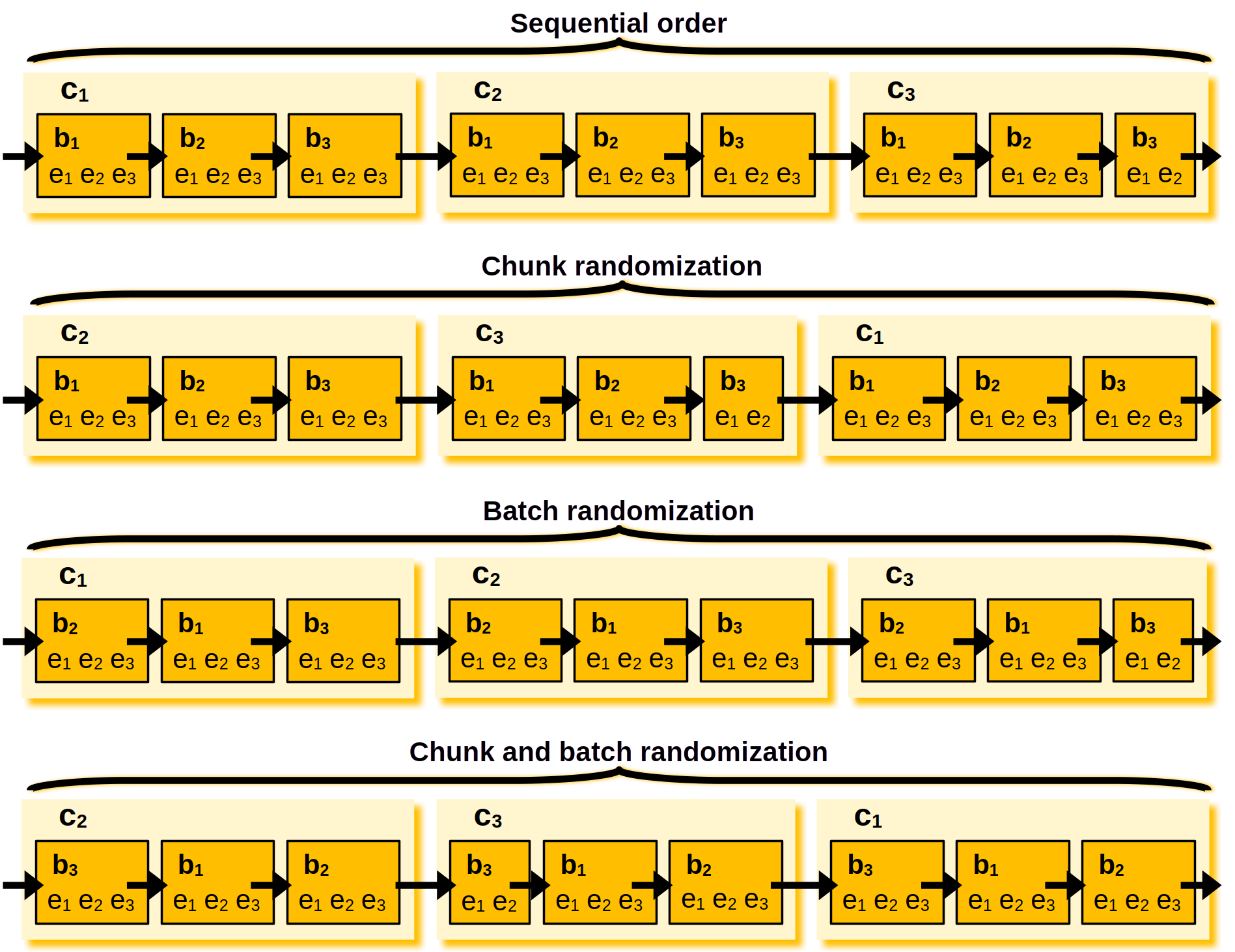
Visualization of the randomization strategies that can be used with the offline sequencer. The \(c_i\) is read as the i-th chunk, \(b_j\) as the j-th batch, and \(e_k\) as the k-th element. The sequencing starts on the left side and moves towards the right side.

The JSON below shows an example of how to configure a DLOfflineSequencer wrapping a DLSequencer (see deep learning sequencer documentation).

"training_sequencer": {
    "type": "DLOfflineSequencer",
    "offline_storage": "/tmp/training_dataset.os1",
    "chunk_size": 250,
    "chunk_randomization": false,
    "batch_randomization": false,
    "disable_offline_storage_writing": false,
    "offline_pcloud": [
        "/data/point_clouds/pcloud2.laz",
        "/data/point_clouds/pcloud3.laz"
    ],
    "backbone": {
        "type": "DLSequencer",
        "random_shuffle_indices": false,
        "augmentor": {
            "transformations": [
                    {
                        "type": "Rotation",
                        "axis": [0, 0, 1],
                        "angle_distribution": {
                            "type": "uniform",
                            "start": -3.141592,
                            "end": 3.141592
                        }
                    },
                    {
                        "type": "Scale",
                        "scale_distribution": {
                            "type": "uniform",
                            "start": 0.99,
                            "end": 1.01
                        }
                    },
                    {
                        "type": "Jitter",
                        "noise_distribution": {
                            "type": "normal",
                            "mean": 0,
                            "stdev": 0.001
                        }
                    }
            ]
        }
    }
}

The JSON above specifies an offline sequencer that considers the point cloud in the current pipeline but also two other point clouds to generate an offline data storage. It uses a chunk size of 250 batches with no randomization at all.

Arguments

– type

The type of sequencer to be used. It must be "DLOfflineSequencer" to use a DLOfflineSequencer.

– offline_storage

The path to the file where the offline storage will be written (and read).

– chunk_size

How many batches per chunk.

– chunk_randomization

Whether to randomize the order in which the chunks are iterated (true) or not (false).

– batch_randomization

Whether to randomize the order in which the batches are iterated (true) or not (false).

– disable_offline_storage_writing

Whether to allow writing to the storage file (false) or not (true). Disable writing can be especially useful to load a previously written offline storage without extending it with further data.

– offline_pcloud

A list with paths to extra point clouds to be pre-processed and included into the offline storage. Note that only the deep learning pre-processor will be applied, i.e., previous components of the pipeline that have updated the input point cloud will not be applied to these point clouds. Therefore, it is strongly recommended to use offline sequencers only with pipelines that do not apply any other pre-processing to the point clouds besides the one defined for the neural network.

– backbone

The specification of the decorated sequencer. For example, it can be a deep learning sequencer.

Training paradigms

Continual learning

Once a model has been trained, it might be the case that we want to train it using a different dataset. Using more training data on a model is likely to improve its generalization capabilities. In the VL3D framework, further training of a pretrained model is quite simple. Using the pretrained_model element inside a training component to specify the path to a pretrained model is enough, as shown in the JSON below:

{
    "train": "PointNetPwiseClassifier",
    "pretrained_model": "out/my_model/pipe/MyModel.model"
}

The JSON above loads a pretrained PointNetPwiseClassif model for further training. Note that model parameters are available. For example, it is possible to change the optimization of the model through the compilation_args element. This can be used to start the training at a lower learning rate than the original model to avoid losing what has been learned before, as typical in fine-tuning. Alternatively, the pretrained_nn_path element can be set to specify the path to the .keras file corresponding to the model. This specification is useful when the path to the files has changed and they cannot be found without the explicit paths.

Transfer learning

Transfer learning is often carried out by transferring the weights of a source model \(A\) to a target model \(B\). The "transfer_weights" list can be defined inside the "model_handling" specification of a deep learning model to govern what weights of \(A\) are transferred to what layers of \(B\). The transferring domain is the entire layer, i.e., the weights from a layer \(A_l\) are transferred to the weights of a layer \(B_l\) that must be compatible in terms of number of tensors representing weights and the dimensionality of the tensors. See DLTransferHandler for further details.

The JSON below shows how a "transfer_weights" list can be defined inside a "model_handling" specification:

"transfer_weights": [
    {
        "model_weights": "/oldext4/lidar_data/vl3dhack/multiclass/out/DL_SFLNETPP/T5/model/SFLNET.keras",
        "layer_translator": {
            "PreHG_d4_5": null,
            "LightKPConv_d4_5": null,
            "LightKPConv_d4_5_BN": null,
            "LightKPConv_d4_5_ReLU": null,
            "PostHG_d4_5": null,
            "ParHG_d4_5": null,
            "PostHG_d4_5_BN": null,
            "PostHG_d4_5_ACT": null,
            "PreHG_d5_6": null,
            "LightKPConv_d5_6": null,
            "LightKPConv_d5_6_BN": null,
            "LightKPConv_d5_6_ReLU": null,
            "PostHG_d5_6": null,
            "ParHG_d5_6": null,
            "PostHG_d5_6_BN": null,
            "PostHG_d5_6_ACT": null
        },
        "default_to_null": false
    }
]

The JSON above defines a transfer between two SFL-Net models. The target model will accept most weights from the source model. Only the weights of feature extraction layers in the encoding hierarchy at depth five and four will be initialized from scratch.

Arguments

– transfer_weights

A list specifying the many transfer operations that must be carried out. Note that the transferrings will occur in the same order they are given. Thus, if a layer is transferred more than once, only the last time will define the actual weights for the target model.

– model_weights

A path to either a .keras file containing a full keras model or a .weights.h5 file containing only the weights of a keras model.

– layer_translator

Dictionary whose keys represent the original name of a layer in the target model and whose keys give the corresponding name in the domain of the source model. Note that when a .keras file is given, the names of the layers correspond to those that appear in the model summary. However, when a .weights.h5 file is given, the names of the layers are given by the snake-formatted class name for the first occurence of the layer. Further repetitions append _1, _2, _3 and so on. The alternative name format for the .weights.h5 is due to how keras automatically renames its layers for weights-only serialization. Users are strongly encouraged to use .keras files for transfer learning as they are less prone to errors and future problems.

– default_to_null

Boolean flag governing whether to assume as null those target layers who do not appear on the translator. If the flag is set to true and there is no key in the translator matching the target layer name, then that layer will be initialized from scratch. If the flat is set to false (default), the name of the target layer will be assume to be same as the name of the source layer.

Freezing layers

Sometimes it might be interesting to freeze some layers during training, i.e., to avoid updating their weights (parameters) when training a neural network. For example, hierarchical feature extraction architectures often compute the most general features on the less deep levels of the hierarchy. Thus, it makes sense to freeze these layers and retrain only the deepest levels to tune the model on a new dataset. Moreover, freeze training can be especially useful when combined with transfer learning. One typical practice is to transfer the hierarchical feature extraction layers of a model and freeze them so they are used as a backbone. One could add new layers on top of the backbone or unfreeze only the final ones doing the classification itself. This way the new model can exploit the features from a pretrained model but adapting to a different task. See DLTrainingHandler for further details.

The JSON below shows how a "freeze_training" list can be defined inside a "model_handling" specification:

"freeze_training": [
    {
        "layers": [
            "PreHG_d1_1", "LightKPConv_d1_1", "LightKPConv_d1_1_BN", "LightKPConv_d1_1_ReLU", "PostHG_d1_1", "ParHG_d1_1", "PostHG_d1_1_BN", "PostHG_d1_1_ACT",
            "PreHG_d1_2", "LightKPConv_d1_2", "LightKPConv_d1_2_BN", "LightKPConv_d1_2_ReLU", "PostHG_d1_2", "ParHG_d1_2", "PostHG_d1_2_BN", "PostHG_d1_2_ACT"
        ],
        "initial_learning_rate": 1e-3,
        "training_interval": [5, -1],
        "strategy": null
    },
]

The JSON above specified that the layers at the first depth of a hierarchical feature extractor must be frozen after the fifth iteration. At the same time, the learning rate will be restarted to \(10^{-3}\) and the layers will remain frozen until the end of training.

Arguments

– freeze_training

A list specifying the many freeze operations that must be carried out.

– layers

A list with the names of the layers to freeze. Alternatively, it can be the string "all" to consider all the layers in sequential order or "all_reverse" to consider them in reverse sequential order.

– initial_learning_rate

The initial learning rate for the training process with the specified frozen layers. If null, the learning rate will be the corresponding one continuing the previous training process, i.e., next iteration of the current scheduler.

– training_interval

The epoch interval during which the layers must remain frozen. It is given as a list of two values. The first one is the epoch at which the freeze starts. The last one is the epoch at which it ends. Note that for the end point it is possible to use -1 which means the layer will be unfrozen at the end of all training epochs.

– strategy

The strategy to be applied. It can be null, which means no special strategy will be applied (the layers are frozen during the given interval).

– type

What type of strategy must be used. It can be "round_robin" (a subset of the layers is frozen and this subset changes after a given number of epochs selecting consecutive layers cyclically) or "random" (a random subset of the layers is frozen and this subset changes after a given number of epochs).

– iterative_span

The number of epochs that the subset of layers selected by the strategy lasts until it is updated.

– window_size

How many layers from the pool of layers (layers) are considered for the subset of layers to be frozen by the specified strategy.

To understand how the round robin strategy works, assume a model with five layers \(A, B, C, D, E\). Let us say that we consider a round robin strategy with an iterative span of five and a window size of two. First, the layers \(A\) and \(B\) will be frozen for five epochs. Afterward, layers \(A\) and \(B\) will become unfrozen but layers \(C\) and \(D\) will be frozen. Then, layers \(C\) and \(D\) will be unfrozen but layer \(E\) will be frozen. Next, layer \(D\) will become unfrozen and layers \(A\) and \(B\) will be frozen again, and so on until the end of training.

TORF training tools

The TransfOctoRF model (TransfOctoRFClassificationModel, "train": "TransfOctoRFClassifier") is an orchestrator that wraps a C++ Random Forest with a Keras neural network. The three training tools described above (continual learning, transfer learning, and freezing layers) are also supported by its neural-network stage, with the same semantics and JSON syntax. There are two TORF-specific aspects to keep in mind:

1. Continual learning uses the standard pretrained_model key. When a previously trained TORF model is loaded for further training, the orchestrator detects that a fitted neural network is already present and reuses it instead of rebuilding the architecture (which would discard the weights). Any keys nested under nn_hparams in the new specification are merged on top of the stored hyperparameters, so partial overrides such as {"epochs": 30} work as expected.

2. Transfer learning and freezing layers are configured through two TORF-specific top-level keys, nn_transfer_weights and nn_freeze_training, that live as siblings of ``nn_hparams`` in the TORF specification (not nested inside nn_hparams). The value format inside each entry is identical to the standard transfer_weights and freeze_training specifications described above.

See TORFTransferHandler (the TORF-specific subclass of DLTransferHandler) and DLFreezeTrainingExecutor (the shared engine that drives freeze-training schedules for both the standard deep learning stack and the TORF NN). The TORF NN handler itself is TransfOctoRFHandler.

The JSON below shows a TORF specification that uses all three training tools at once: continue training from a serialized TORF model, transfer the lower layers of a different pretrained network, and freeze the output classifier head during the first five epochs.

{
    "train": "TransfOctoRFClassifier",
    "pretrained_model": "out/torf_v1/pipe/torf.model",
    "nn_transfer_weights": [
        {
            "model_weights": "out/torf_v0/pipe/nn.keras",
            "layer_translator": {
                "out": null
            },
            "default_to_null": false
        }
    ],
    "nn_freeze_training": [
        {
            "layers": ["out"],
            "initial_learning_rate": 1e-3,
            "training_interval": [0, 5],
            "strategy": null
        }
    ],
    "nn_hparams": {
        "operator": "transformer",
        "epochs": 50,
        "learning_rate": 0.001
    }
}

Arguments

– nn_transfer_weights

A list specifying the transfer operations applied to the TORF neural network before training. Each entry follows the exact same schema as a transfer_weights entry (see above): model_weights, layer_translator, and default_to_null.

– nn_freeze_training

A list specifying the freeze-training schedule applied to the TORF neural network during training. Each entry follows the exact same schema as a freeze_training entry (see above): layers, initial_learning_rate, training_interval, and strategy.

– preserve_optimizer_state

Optional boolean. Defaults to false. When false (default), the NN optimizer (Adam moments, learning-rate scheduler iteration counter, etc.) is stripped at the end of training to save approximately twice the model size of RAM (appropriate for the common train-then-predict workflow where the optimizer is no longer needed once training completes). When true, the optimizer is retained and persisted alongside the model weights through pickle, so a subsequent continue-training pass (via pretrained_model) resumes the LR schedule and Adam moments from where the original training left off rather than re-initializing them. Set true whenever you intend to reload the saved model for additional NN training and want the optimizer state to carry over (typical for stateful schedules such as cosine or exponential decay).

Note

The flag must be set during the training run whose save you want to contain the optimizer. Setting it on a continue-training spec (via pretrained_model) only affects subsequent saves: if the checkpoint being loaded was produced with preserve_optimizer_state=false, its .keras archive does not contain optimizer state and the next training pass will rebuild the optimizer from scratch regardless of the new flag value. The optimizer carries forward correctly when the same flag value is used for both the run that produced the checkpoint and any downstream continue-training runs that re-save.

Note

When continuing training with a pretrained_model, omitting nn_transfer_weights or nn_freeze_training from the new specification keeps the corresponding value from the saved model rather than clearing it. The orchestrator tracks that the saved model already received its initial transfer at the original training time, so the next training pass does not re-apply the transfer over the already-trained weights. Restating the same nn_transfer_weights block in the new specification (e.g., for self-documentation purposes) is also a no-op. The orchestrator compares the new spec against the saved one and only rebuilds the transfer handler when they differ. To disable a previously configured tool while continuing training, explicitly set its key to null in the new JSON specification. To re-apply transfer learning from a different source (or with a different layer translator), pass a new nn_transfer_weights spec whose contents differ from the saved one; the orchestrator rebuilds the transfer handler so the new transfer fires on the next training pass.

Working examples

This section contains many simply working examples that provide a simple baseline configuration for some of the different models that can be designed with the VirtuaLearn3D++ framework.

PointNet-like model

This example shows how to define two different pipelines, one to train a model and export it as a PredictivePipeline, the other to use the predictive pipeline to compute a semantic segmentation on a previously unseen point cloud. Readers are referred to the pipelines documentation to read more about how pipelines work and to see more examples.

Training pipeline

The training pipeline will train a PointNetPwiseClassif to classify the points depending on whether they represent the ground, vegetation, buildings, urban furniture, or vehicles. The training point cloud is generated from the March 2018 training point cloud in the Hessigheim dataset by reducing the original classes to the five categories mentioned before.

The receptive fields are computed following a furthest point subsampling strategy such that each receptive field has \(8192\) points. The receptive fields are built from rectangular neighborhoods with a half size (radius) of \(5\,\mathrm{m}\), i.e., voxels with edge length \(10\,\mathrm{m}\). Furthermore, a class weighting strategy is used to modify the loss function so it accounts for the class imbalance. In this case, the ground class has a weight of \(\frac{1}{4}\), the vegetation and building classes a weight of \(\frac{1}{2}\), and the urban furniture and vehicle classes a weight of one.

The learning rate on plateau strategy is configured with a highly enough patience so it will never trigger. However, as it is enabled, the learning rate will be traced by the training history and included in the plots. The optimizer is a stochastic gradient descent (SGD) initialized with a learning rate of \(10^{-2}\). The learning rate will be exponentially reduced with a decay rate of \(0.96\) each \(2000\) steps. Once the training has been finished, the model will be exported to a predictive pipeline that includes the class transformation so it can be directly applied later to the corresponding validation point cloud in the Hessigheim dataset.

The JSON below corresponds to the described training pipeline.

{
  "in_pcloud": [
    "/data/Hessigheim_Benchmark/Epoch_March2018/LiDAR/Mar18_train.laz"
  ],
  "out_pcloud": [
    "/data/Hessigheim_Benchmark/Epoch_March2018/vl3d/out/Rect3D_alt_5m_T1/*"
  ],
  "sequential_pipeline": [
    {
        "class_transformer": "ClassReducer",
        "on_predictions": false,
        "input_class_names": ["Low vegetation", "Impervious surface", "Vehicle", "Urban furniture", "Roof", "Facade", "Shrub", "Tree", "Soil/Gravel", "Vertical surface", "Chimney"],
        "output_class_names": ["Ground", "Vegetation", "Building", "Urban furniture", "Vehicle"],
        "class_groups": [["Low vegetation", "Impervious surface", "Soil/Gravel"], ["Shrub", "Tree"], ["Roof", "Facade", "Vertical surface", "Chimney"], ["Urban furniture"], ["Vehicle"]],
        "report_path": "*class_reduction.log",
        "plot_path": "*class_reduction.svg"
    },
    {
      "train": "PointNetPwiseClassifier",
      "fnames": ["AUTO"],
      "training_type": "base",
      "random_seed": null,
      "model_args": {
        "num_classes": 5,
        "class_names": ["Ground", "Vegetation", "Building", "Urban furniture", "Vehicle"],
        "num_pwise_feats": 20,
        "pre_processing": {
            "pre_processor": "furthest_point_subsampling",
            "to_unit_sphere": false,
            "support_strategy": "grid",
            "support_chunk_size": 2000,
            "support_strategy_fast": false,
            "center_on_pcloud": true,
            "num_points": 8192,
            "num_encoding_neighbors": 1,
            "fast": false,
            "neighborhood": {
                "type": "rectangular3D",
                "radius": 5.0,
                "separation_factor": 0.8
            },
            "nthreads": 12,
            "training_receptive_fields_distribution_report_path": "*/training_eval/training_receptive_fields_distribution.log",
            "training_receptive_fields_distribution_plot_path": "*/training_eval/training_receptive_fields_distribution.svg",
            "training_receptive_fields_dir": "*/training_eval/training_receptive_fields/",
            "receptive_fields_distribution_report_path": "*/training_eval/receptive_fields_distribution.log",
            "receptive_fields_distribution_plot_path": "*/training_eval/receptive_fields_distribution.svg",
            "receptive_fields_dir": "*/training_eval/receptive_fields/",
            "training_support_points_report_path": "*/training_eval/training_support_points.las",
            "support_points_report_path": "*/training_eval/support_points.las"
        },
        "kernel_initializer": "he_normal",
        "pretransf_feats_spec": [
            {
                "filters": 64,
                "name": "prefeats64_A"
            },
            {
                "filters": 64,
                "name": "prefeats_64B"
            },
            {
                "filters": 128,
                "name": "prefeats_128"
            },
            {
                "filters": 192,
                "name": "prefeats_192"
            }
        ],
        "postransf_feats_spec": [
            {
                "filters": 128,
                "name": "posfeats_128"
            },
            {
                "filters": 192,
                "name": "posfeats_192"
            },
            {
                "filters": 256,
                "name": "posfeats_end_64"
            }
        ],
        "tnet_pre_filters_spec": [64, 128, 192],
        "tnet_post_filters_spec": [192, 128, 64],
        "final_shared_mlps": [256, 192, 128],
        "skip_link_features_X": false,
        "include_pretransf_feats_X": false,
        "include_transf_feats_X": true,
        "include_postransf_feats_X": false,
        "include_global_feats_X": true,
        "skip_link_features_F": false,
        "include_pretransf_feats_F": false,
        "include_transf_feats_F": false,
        "include_postransf_feats_F": false,
        "include_global_feats_F": false,
        "model_handling": {
            "summary_report_path": "*/model_summary.log",
            "training_history_dir": "*/training_eval/history",
            "features_structuring_representation_dir": "*/training_eval/feat_struct_layer/",
            "class_weight": [0.25, 0.5, 0.5, 1, 1],
            "training_epochs": 200,
            "batch_size": 16,
            "checkpoint_path": "*/checkpoint.weights.h5",
            "checkpoint_monitor": "loss",
            "learning_rate_on_plateau": {
                "monitor": "loss",
                "mode": "min",
                "factor": 0.1,
                "patience": 2000,
                "cooldown": 5,
                "min_delta": 0.01,
                "min_lr": 1e-6
            }
        },
        "compilation_args": {
            "optimizer": {
                "algorithm": "SGD",
                "learning_rate": {
                    "schedule": "exponential_decay",
                    "schedule_args": {
                        "initial_learning_rate": 1e-2,
                        "decay_steps": 2000,
                        "decay_rate": 0.96,
                        "staircase": false
                    }
                }
            },
            "loss": {
                "function": "class_weighted_categorical_crossentropy"
            },
            "metrics": [
                "categorical_accuracy"
            ]
        },
        "architecture_graph_path": "*/model_graph.png",
        "architecture_graph_args": {
            "show_shapes": true,
            "show_dtype": true,
            "show_layer_names": true,
            "rankdir": "TB",
            "expand_nested": true,
            "dpi": 300,
            "show_layer_activations": true
        }
      },
      "autoval_metrics": ["OA", "P", "R", "F1", "IoU", "wP", "wR", "wF1", "wIoU", "MCC", "Kappa"],
      "training_evaluation_metrics": ["OA", "P", "R", "F1", "IoU", "wP", "wR", "wF1", "wIoU", "MCC", "Kappa"],
      "training_class_evaluation_metrics": ["P", "R", "F1", "IoU"],
      "training_evaluation_report_path": "*/training_eval/evaluation.log",
      "training_class_evaluation_report_path": "*/training_eval/class_evaluation.log",
      "training_confusion_matrix_report_path": "*/training_eval/confusion.log",
      "training_confusion_matrix_plot_path": "*/training_eval/confusion.svg",
      "training_class_distribution_report_path": "*/training_eval/class_distribution.log",
      "training_class_distribution_plot_path": "*/training_eval/class_distribution.svg",
      "training_classified_point_cloud_path": "*/training_eval/classified_point_cloud.las",
      "training_activations_path": "*/training_eval/activations.las"
    },
    {
      "writer": "PredictivePipelineWriter",
      "out_pipeline": "*pipe/Rect3D_5m_T1.pipe",
      "include_writer": false,
      "include_imputer": false,
      "include_feature_transformer": false,
      "include_miner": false,
      "include_class_transformer": true
    }
  ]
}

The table below represents the distribution of reference and predicted labels on the training dataset. The class imbalance can be clearly observed. Nevertheless, thanks to the class weights, the model gives more importance to the less populated classes, so they have an appreciable impact on the weight updates during the gradient descent iterations.

CLASS	PRED. COUNT	PRED. PERCENT.	TRUE COUNT	TRUE PERCENT.
Ground	39676955	66.746	40385955	67.938
Vegetation	9858128	16.584	9163959	15.416
Building	8257266	13.891	8477955	14.262
Urban furniture	1367284	2.300	1159205	1.950
Vehicle	285473	0.480	258032	0.434

The figure below represents the receptive fields. The top rows represent the outputs of the softmax layer that describe from zero to one how likely a given point is to belong to the corresponding class. The bottom row represents the reference (classification) and predicted (predictions) labels inside the receptive field.

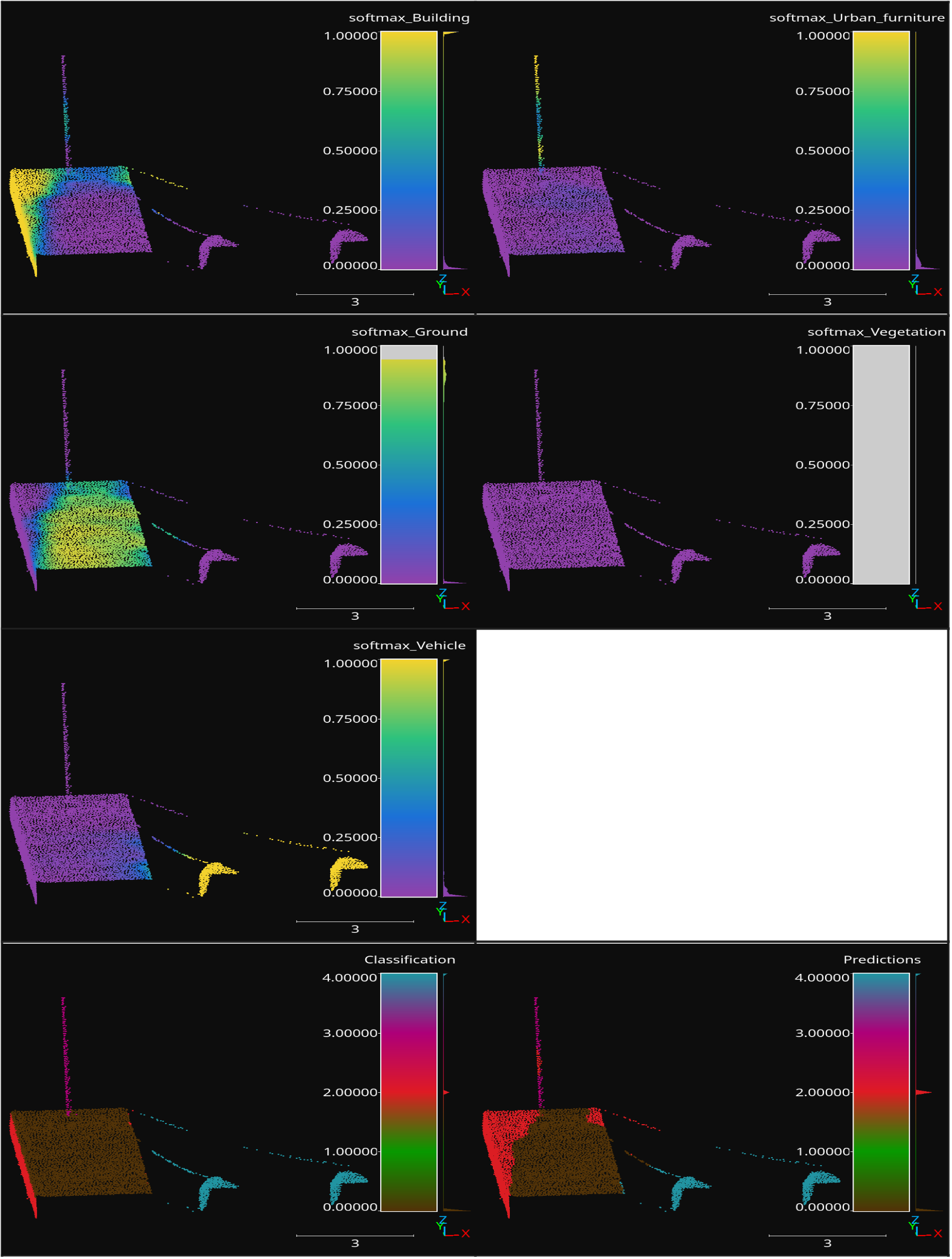
Visualization of a receptive field from a trained PointNet-based classifier. The softmax representation uses a color map from zero (violet) to one (yellow). The classification (reference labels) and predictions use the same color code for the classes.

Predictive pipeline

The predictive pipeline will use the model trained on the first point cloud to compute an urban semantic segmentation on a validation point cloud. More concretely, the validation point cloud corresponds to the March 2018 epoch of the Hessigheim dataset.

The predictions will be exported through the ClassifiedPcloudWriter, which means the boolean mask on success and fail will be available. Also, the ClassificationEvaluator will be used to quantify the quality of the predictions through many evaluation metrics.

The JSON below corresponds to the described predictive pipeline.

{
  "in_pcloud": [
    "/data/Hessigheim_Benchmark/Epoch_March2018/LiDAR/Mar18_val.laz"
  ],
  "out_pcloud": [
    "/data/Hessigheim_Benchmark/Epoch_March2018/vl3d/out/Rect3D_alt_5m_T1/validation_rfsep0_4/*"
  ],
  "sequential_pipeline": [
    {
      "predict": "PredictivePipeline",
      "model_path": "/data/Hessigheim_Benchmark/Epoch_March2018/vl3d/out/Rect3D_alt_5m_T1/pipe/Rect3D_5m_T1.pipe"
    },
    {
        "writer": "ClassifiedPcloudWriter",
        "out_pcloud": "*predicted.las"
    },
    {
      "writer": "PredictionsWriter",
      "out_preds": "*predictions.lbl"
    },
    {
      "eval": "ClassificationEvaluator",
      "class_names": ["Ground", "Vegetation", "Building", "Urban furniture", "Vehicle"],
      "metrics": ["OA", "P", "R", "F1", "IoU", "wP", "wR", "wF1", "wIoU", "MCC", "Kappa"],
      "class_metrics": ["P", "R", "F1", "IoU"],
      "report_path": "*report/global_eval.log",
      "class_report_path": "*report/class_eval.log",
      "confusion_matrix_report_path" : "*report/confusion_matrix.log",
      "confusion_matrix_plot_path" : "*plot/confusion_matrix.svg",
      "class_distribution_report_path": "*report/class_distribution.log",
      "class_distribution_plot_path": "*plot/class_distribution.svg"
    }
  ]
}

The table below represents the class-wise evaluation metrics. It shows the precision, recall, F1-score, and intersection over union (IoU) for each class. It can be seen that the more populated classes, ground, vegetation, and building yield the best results, while the less frequent classes yield worse results, as expected.

CLASS	P	R	F1	IoU
Ground	96.422	94.760	95.584	91.542
Vegetation	88.068	88.835	88.450	79.292
Building	85.890	92.726	89.177	80.468
Urban furniture	30.062	26.075	27.927	16.229
Vehicle	67.671	20.389	31.336	18.579

The figure below shows the reference and predicted labels, as well as the fail/success boolean mask representing correctly classified (gray) and misclassified (red) points.

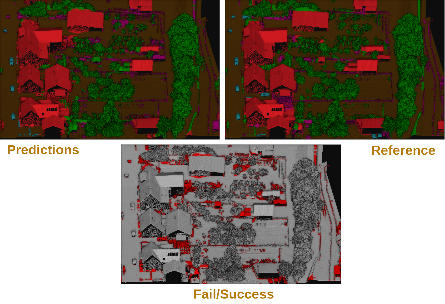
Visualization of the semantic segmentation model applied to previously unseen data. The bottom image shows correctly classified points in gray and misclassified points in red. The predictions and reference images use the same color code for the classes.

PointNet++-based model

This example shows how to define two different pipelines, one to train a PointNet++-based model (see PointNet++ documentation) and export it as a PredictivePipeline, the other to use the predictive pipeline to compute a semantic segmentation on a previously unseen point cloud. Readers are referred to the pipelines documentation to read more about how pipelines work and to see more examples.

Training pipeline

The training pipeline will train a ConvAutoencPwiseClassif for the multiclass semantic segmentation of the points. The training point cloud is generated from the March 2018 training point cloud in the Hessigheim dataset by transforming the RGB color components to its HSV representation with HSV from RGB miner.

Note that this model is drastically different compared to the standard PointNet++ architecture (closer to what is shown in the PointNet++ documentation). Thus, this example shows how the VL3D++ framework can be used to update the architecture of an older feature extractor to achieve much better results. In this case, the main difference lies in the use of hourglass blocks for wrapping the PointNet-based feature extractors and also as upsampling layers.

The JSON below corresponds to the commented training pipeline.

{
    "in_pcloud": [
        "/ext4/hei/Hessigheim_Benchmark/Epoch_March2018/vl3d/mined/Mar18_train_hsv_std.laz"
    ],
    "out_pcloud": [
        "/ext4/hei/Hessigheim_Benchmark/Epoch_March2018/vl3d/out/pnetpp_hourglass/T1/*"
    ],
    "sequential_pipeline": [
        {
            "train": "ConvolutionalAutoencoderPwiseClassifier",
            "training_type": "base",
            "fnames": ["ones", "HSV_Hrad", "HSV_S", "HSV_V"],
            "random_seed": null,
            "model_args": {
                "fnames": ["ones", "HSV_Hrad", "HSV_S", "HSV_V"],
                "num_classes": 11,
                "class_names": ["LowVeg", "ImpSurf", "Vehicle", "UrbanFurni", "Roof", "Facade", "Shrub", "Tree", "Soil/Gravel", "VertSurf", "Chimney"],
                "pre_processing": {
                    "pre_processor": "hierarchical_fpspp",
                    "support_strategy_num_points": 25000,
                    "to_unit_sphere": false,
                    "support_strategy": "fps",
                    "support_strategy_fast": 2,
                    "min_distance": 0.03,
                    "receptive_field_oversampling": {
                        "min_points": 2,
                        "strategy": "nearest",
                        "k": 3,
                        "radius": 0.5
                    },
                    "center_on_pcloud": true,
                    "training_class_distribution": [2250, 2250, 2250, 2250, 2250, 2250, 2250, 2250, 2250, 2250, 2250],
                    "neighborhood": {
                        "type": "sphere",
                        "radius": 5.0,
                        "separation_factor": 0.8
                    },
                    "num_points_per_depth": [4096, 1024, 256, 64, 16],
                    "fast_flag_per_depth": [4, 4, false, false, false],
                    "num_downsampling_neighbors": [1, 16, 16, 16, 16],
                    "num_pwise_neighbors": [16, 16, 16, 16, 16],
                    "num_upsampling_neighbors": [1, 16, 16, 16, 16],
                    "nthreads": -1,
                    "training_receptive_fields_distribution_report_path": null,
                    "training_receptive_fields_distribution_plot_path": null,
                    "training_receptive_fields_dir": null,
                    "receptive_fields_distribution_report_path": null,
                    "receptive_fields_distribution_plot_path": null,
                    "receptive_fields_dir": null,
                    "training_support_points_report_path": null,
                    "support_points_report_path": null
                },
                "feature_extraction": {
                    "type": "PointNet",
                    "operations_per_depth": [2, 1, 1, 1, 1],
                    "feature_space_dims": [64, 64, 128, 256, 512, 1024],
                    "bn": true,
                    "bn_momentum": 0.95,
                    "H_activation": ["relu", "relu", "relu", "relu", "relu", "relu"],
                    "H_initializer": ["he_uniform", "he_uniform", "he_uniform", "he_uniform", "he_uniform", "he_uniform"],
                    "H_regularizer": [null, null, null, null, null, null],
                    "H_constraint": [null, null, null, null, null, null],
                    "gamma_activation": ["relu", "relu", "relu", "relu", "relu", "relu"],
                    "gamma_kernel_initializer": ["he_uniform", "he_uniform", "he_uniform", "he_uniform", "he_uniform", "he_uniform"],
                    "gamma_kernel_regularizer": [null, null, null, null, null, null],
                    "gamma_kernel_constraint": [null, null, null, null, null, null],
                    "gamma_bias_enabled": [true, true, true, true, true, true],
                    "gamma_bias_initializer": ["zeros", "zeros", "zeros", "zeros", "zeros", "zeros"],
                    "gamma_bias_regularizer": [null, null, null, null, null, null],
                    "gamma_bias_constraint": [null, null, null, null, null, null],
                    "activate": true,
                    "hourglass_wrapper": {
                        "internal_dim": [2, 2, 4, 16, 32, 64],
                        "parallel_internal_dim": [8, 8, 16, 32, 64, 128],
                        "activation": ["relu", "relu", "relu", "relu", "relu", "relu"],
                        "activation2": [null, null, null, null, null, null],
                        "regularize": [true, true, true, true, true, true],
                        "W1_initializer": ["he_uniform", "he_uniform", "he_uniform", "he_uniform", "he_uniform", "he_uniform"],
                        "W1_regularizer": [null, null, null, null, null, null],
                        "W1_constraint": [null, null, null, null, null, null],
                        "W2_initializer": ["he_uniform", "he_uniform", "he_uniform", "he_uniform", "he_uniform", "he_uniform"],
                        "W2_regularizer": [null, null, null, null, null, null],
                        "W2_constraint": [null, null, null, null, null, null],
                        "loss_factor": 0.1,
                        "subspace_factor": 0.125,
                        "feature_dim_divisor": 4,
                        "bn": false,
                        "bn_momentum": 0.95,
                        "out_bn": true,
                        "out_bn_momentum": 0.95,
                        "out_activation": "relu"
                    }
                },
                "features_alignment": null,
                "downsampling_filter": "mean",
                "upsampling_filter": "mean",
                "upsampling_bn": true,
                "upsampling_momentum": 0.95,
                "upsampling_hourglass": {
                    "activation": "relu",
                    "activation2": null,
                    "regularize": true,
                    "W1_initializer": "he_uniform",
                    "W1_regularizer": null,
                    "W1_constraint": null,
                    "W2_initializer": "he_uniform",
                    "W2_regularizer": null,
                    "W2_constraint": null,
                    "loss_factor": 0.1,
                    "subspace_factor": 0.125
                },
                "conv1d": true,
                "conv1d_kernel_initializer": "he_uniform",
                "neck":{
                    "max_depth": 2,
                    "hidden_channels": [64, 64],
                    "kernel_initializer": ["he_uniform", "he_uniform"],
                    "kernel_regularizer": [null, null],
                    "kernel_constraint": [null, null],
                    "bn_momentum": [0.95, 0.95],
                    "activation": ["relu", "relu"]
                },
                "output_kernel_initializer": "he_normal",
                "model_handling": {
                    "summary_report_path": "*/model_summary.log",
                    "training_history_dir": "*/training_eval/history",
                    "class_weight": [1.0, 1.0, 1.0, 1.0, 1.0, 1.0, 1.0, 1.0, 1.0, 1.0, 1.0],
                    "training_epochs": 200,
                    "batch_size": 16,
                    "training_sequencer": {
                        "type": "DLSequencer",
                        "random_shuffle_indices": true,
                        "augmentor": {
                            "transformations": [
                                    {
                                        "type": "Rotation",
                                        "axis": [0, 0, 1],
                                        "angle_distribution": {
                                            "type": "uniform",
                                            "start": -3.141592,
                                            "end": 3.141592
                                        }
                                    },
                                    {
                                        "type": "Scale",
                                        "scale_distribution": {
                                            "type": "uniform",
                                            "start": 0.985,
                                            "end": 1.015
                                        }
                                    },
                                    {
                                        "type": "Jitter",
                                        "noise_distribution": {
                                            "type": "normal",
                                            "mean": 0,
                                            "stdev": 0.0033
                                        }
                                    }
                            ]
                        }
                    },
                    "prediction_reducer": {
                        "reduce_strategy" : {
                            "type": "MeanPredReduceStrategy"
                        },
                        "select_strategy": {
                            "type": "ArgMaxPredSelectStrategy"
                        }
                    },
                    "checkpoint_path": "*/checkpoint.weights.h5",
                    "checkpoint_monitor": "loss",
                    "learning_rate_on_plateau": {
                        "monitor": "loss",
                        "mode": "min",
                        "factor": 0.1,
                        "patience": 2000,
                        "cooldown": 5,
                        "min_delta": 0.01,
                        "min_lr": 1e-6
                    }
                },
                "compilation_args": {
                    "optimizer": {
                        "algorithm": "AdamW",
                        "learning_rate": {
                            "schedule": "exponential_decay",
                            "schedule_args": {
                                "initial_learning_rate": 1e-2,
                                "decay_steps": 2500,
                                "decay_rate": 0.96,
                                "staircase": false
                            }
                        }
                    },
                    "loss": {
                        "function": "class_weighted_categorical_crossentropy"
                    },
                    "metrics": [
                        "categorical_accuracy",
                        "f1"
                    ]
                },
                "architecture_graph_path": "*/model_graph.png",
                "architecture_graph_args": {
                    "show_shapes": true,
                    "show_dtype": true,
                    "show_layer_names": true,
                    "rankdir": "TB",
                    "expand_nested": true,
                    "dpi": 300,
                    "show_layer_activations": true
                }
            },
            "autoval_metrics": null,
            "training_evaluation_metrics": null,
            "training_class_evaluation_metrics": null,
            "training_evaluation_report_path": null,
            "training_class_evaluation_report_path": null,
            "training_confusion_matrix_report_path": null,
            "training_confusion_matrix_plot_path": null,
            "training_class_distribution_report_path": null,
            "training_class_distribution_plot_path": null,
            "training_classified_point_cloud_path": null,
            "training_activations_path": null
        },
        {
            "writer": "PredictivePipelineWriter",
            "out_pipeline": "*/model/PNetPP.pipe",
            "include_writer": false,
            "include_imputer": true,
            "include_feature_transformer": true,
            "include_miner": true,
            "include_class_transformer": false,
            "include_clustering": false,
            "ignore_predictions": false
        }
    ]
}

The figure below represents the evolution among the many training epochs of the categorical accuracy, the F1-score, the loss function, and the learning rate.

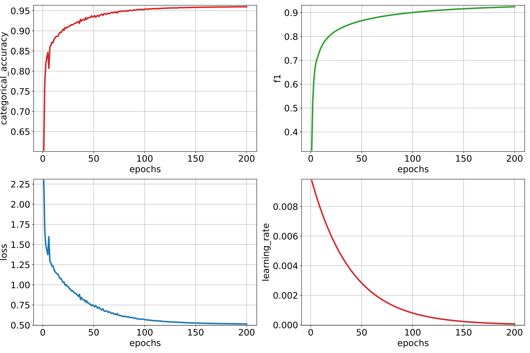
Visualization of the categorical accuracy, the F1-score, the loss function, and the learning rate among \(200\) epochs.

Predictive pipeline

The predictive pipeline will use the model on a validation point cloud from the same dataset and epoch. The predictions will be evaluated through ClassificationEvaluator and they will be exported together with their uncertainties through ClassificationUncertaintyEvaluator.

The JSON below corresponds to the described predictive pipeline.

{
  "in_pcloud": [
    "/ext4/hei/Hessigheim_Benchmark/Epoch_March2018/vl3d/mined/Mar18_val_hsv_std.laz"
  ],
  "out_pcloud": [
    "/ext4/hei/Hessigheim_Benchmark/Epoch_March2018/vl3d/out/pnetpp_hourglass/T1/preds/*"
  ],
  "sequential_pipeline": [
    {
      "predict": "PredictivePipeline",
      "model_path": "/ext4/hei/Hessigheim_Benchmark/Epoch_March2018/vl3d/out/pnetpp_hourglass/T1/model/PNetPP.pipe"
    },
    {
      "eval": "ClassificationEvaluator",
      "class_names": ["LowVeg", "ImpSurf", "Vehicle", "UrbanFurni", "Roof", "Facade", "Shrub", "Tree", "Soil/Gravel", "VertSurf", "Chimney"],
      "metrics": ["OA", "P", "R", "F1", "IoU", "wP", "wR", "wF1", "wIoU", "MCC", "Kappa"],
      "class_metrics": ["P", "R", "F1", "IoU"],
      "confusion_matrix_normalization_strategy": "row",
      "report_path": "*report/global_eval.log",
      "class_report_path": "*report/class_eval.log",
      "confusion_matrix_report_path" : "*report/confusion_matrix.log",
      "confusion_matrix_plot_path" : "*plot/confusion_matrix.svg",
      "class_distribution_report_path": "*report/class_distribution.log",
      "class_distribution_plot_path": "*plot/class_distribution.svg"
    },
    {
        "eval": "ClassificationUncertaintyEvaluator",
        "class_names": ["LowVeg", "ImpSurf", "Vehicle", "UrbanFurni", "Roof", "Facade", "Shrub", "Tree", "Soil/Gravel", "VertSurf", "Chimney"],
        "include_probabilities": true,
        "include_weighted_entropy": false,
        "include_clusters": false,
        "weight_by_predictions": false,
        "num_clusters": 0,
        "clustering_max_iters": 0,
        "clustering_batch_size": 0,
        "clustering_entropy_weights": false,
        "clustering_reduce_function": null,
        "gaussian_kernel_points": 256,
        "report_path": "*uncertainty/uncertainty.las",
        "plot_path": "*uncertainty/"
    }
  ]
}

The table below represents the global evaluation metrics. It shows the overall accuracy (OA), precision (P), recall (R), F1-score (F1), the intersection over union (IoU), all of them weighted by the number of points, the Matthew’s correlation coefficient (MCC), and the Cohen’s Kappa score (Kappa).

OA	P	R	F1	IoU	wP	wR	wF1	wIoU	MCC	Kappa
87.123	81.237	68.394	72.862	60.193	86.649	87.123	86.524	78.050	84.052	84.011

The figure below shows the reference and predicted labels, the class ambiguity as a point-wise uncertainty measurement, and the binary error mask (gray for correctly classified points, red for misclassified ones).

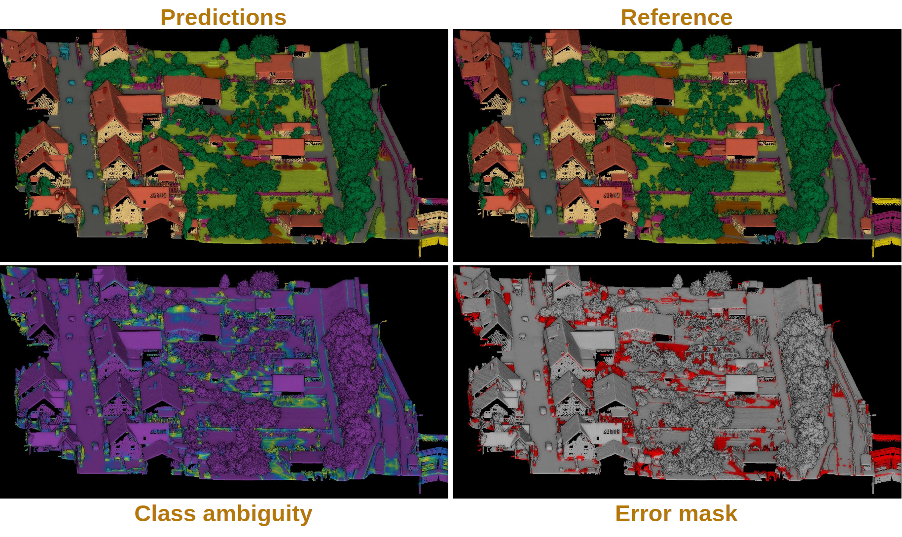
Visualization of the semantic segmentation model applied to previously unseen data. The bottom-right image shows correctly classified points in gray and misclassified points in red. The predictions and reference images use the same color code for the classes. The class ambiguity is represented with purple color for low-uncertainty regions and yellow for high-uncertainty ones.

KPConv-based model

This example shows how to define two different pipelines, one to train a KPConv-based model (see KPConv documentation) and export it as a PredictivePipeline, the other to use the predictive pipeline to compute a semantic segmentation on a previously unseen point cloud. Readers are referred to the pipelines documentation to read more about how pipelines work and to see more examples.

Standardization

The reflectance values in the point clouds considered for this example have been standardized. To reproduce the standardization, build a pipeline with a Standardizer as shown below:

{
    "feature_transformer": "Standardizer",
    "fnames": ["Reflectance", "HSV_Hrad", "HSV_S", "HSV_V"],
    "center": true,
    "scale": true,
    "report_path": "*standardization.log"
}

Finally, add a PredictivePipelineWriter as shown below so the same standardization can be applied to any point cloud later on:

{
  "writer": "PredictivePipelineWriter",
  "out_pipeline": "*STD.pipe",
  "ignore_predictions": true,
  "include_writer": false
  "include_imputer": false,
  "include_feature_transformer": true,
  "include_miner": false,
  "include_class_transformer": false
}

Training pipeline

The training pipeline will train a ConvAutoencPwiseClassif for the multiclass urban semantic segmentation of the points. The training point cloud is the one given in the March 2018 epoch of the Hessigheim dataset . However, its reflectance values have been preprocessed using a Standardizer to have a convenient scale.

The receptive fields are computed following a hierarchical furthest point subsampling strategy such that the hierarchy of receptive field starts with \(512\) points and ends with \(32\). The receptive fields are built from 3D spherical neighborhoods with a radius) of \(3\,\mathrm{m}\).

The first downsampling (i.e., the one that maps the original input neighborhood to the first receptive field) considers only the nearest neighbor. However, the second, third, fourth, and fifth dowsnamplings consider \(16\), \(8\), \(8\), and \(4\) closest neighbors, respectively. The upsampling layers preserve the same number of nearest neighbors. The first neighborhood considered by a KPConv layer knows the \(32\) nearest neighbors instead of only the first one.

The KPConv and strided KPConv layers start with \(64\) output features but end with \(1024\), applying batch normalization during training. The kernels are activated and the influence distance of each kernel point is the same as the kernel radius. Strided kernel point convolutions are used for the downsampling instead of typical faetures downsampling strategies like nearest downsampling, mean, or gaussian RBF.

The JSON below corresponds to the described training pipeline.

{
  "in_pcloud": [
    "/mnt/netapp2/Store_uscciaep/lidar_data/hessigheim/vl3d/mined/Mar18_train_hsv_std.laz"
  ],
  "out_pcloud": [
    "/mnt/netapp2/Store_uscciaep/lidar_data/hessigheim/vl3d/kpconv_R/T1/*"
  ],
  "sequential_pipeline": [
    {
        "train": "ConvolutionalAutoencoderPwiseClassifier",
        "training_type": "base",
        "fnames": ["Reflectance", "ones"],
        "random_seed": null,
        "model_args": {
            "fnames": ["Reflectance", "ones"],
            "num_classes": 11,
            "class_names": ["LowVeg", "ImpSurf", "Vehicle", "UrbanFurni", "Roof", "Facade", "Shrub", "Tree", "Soil/Gravel", "VertSurf", "Chimney"],
            "pre_processing": {
                "pre_processor": "hierarchical_fps",
                "support_strategy_num_points": 60000,
                "to_unit_sphere": false,
                "support_strategy": "fps",
                "support_chunk_size": 2000,
                "support_strategy_fast": true,
                "center_on_pcloud": true,
                "neighborhood": {
                    "type": "sphere",
                    "radius": 3.0,
                    "separation_factor": 0.8
                },
                "num_points_per_depth": [512, 256, 128, 64, 32],
                "fast_flag_per_depth": [false, false, false, false, false],
                "num_downsampling_neighbors": [1, 16, 8, 8, 4],
                "num_pwise_neighbors": [32, 16, 16, 8, 4],
                "num_upsampling_neighbors": [1, 16, 8, 8, 4],
                "nthreads": 12,
                "training_receptive_fields_distribution_report_path": "*/training_eval/training_receptive_fields_distribution.log",
                "training_receptive_fields_distribution_plot_path": "*/training_eval/training_receptive_fields_distribution.svg",
                "training_receptive_fields_dir": null,
                "receptive_fields_distribution_report_path": "*/training_eval/receptive_fields_distribution.log",
                "receptive_fields_distribution_plot_path": "*/training_eval/receptive_fields_distribution.svg",
                "receptive_fields_dir": null,
                "training_support_points_report_path": "*/training_eval/training_support_points.las",
                "support_points_report_path": "*/training_eval/support_points.las"
            },
            "feature_extraction": {
                "type": "KPConv",
                "operations_per_depth": [2, 1, 1, 1, 1],
                "feature_space_dims": [64, 64, 128, 256, 512, 1024],
                "bn": true,
                "bn_momentum": 0.0,
                "activate": true,
                "sigma": [3.0, 3.0, 3.0, 3.0, 3.0, 3.0],
                "kernel_radius": [3.0, 3.0, 3.0, 3.0, 3.0, 3.0],
                "num_kernel_points": [15, 15, 15, 15, 15, 15],
                "deformable": [false, false, false, false, false, false],
                "W_initializer": ["glorot_uniform", "glorot_uniform", "glorot_uniform", "glorot_uniform", "glorot_uniform", "glorot_uniform"],
                "W_regularizer": [null, null, null, null, null, null],
                "W_constraint": [null, null, null, null, null, null]
            },
            "structure_alignment": null,
            "features_alignment": null,
            "downsampling_filter": "strided_kpconv",
            "upsampling_filter": "mean",
            "upsampling_bn": true,
            "upsampling_momentum": 0.0,
            "conv1d_kernel_initializer": "glorot_normal",
            "output_kernel_initializer": "glorot_normal",
            "model_handling": {
                "summary_report_path": "*/model_summary.log",
                "training_history_dir": "*/training_eval/history",
                "kpconv_representation_dir": "*/training_eval/kpconv_layers/",
                "skpconv_representation_dir": "*/training_eval/skpconv_layers/",
                "class_weight": [1, 1, 1, 1, 1, 1, 1, 1, 1, 1, 1],
                "training_epochs": 300,
                "batch_size": 16,
                "checkpoint_path": "*/checkpoint.weights.h5",
                "checkpoint_monitor": "loss",
                "learning_rate_on_plateau": {
                    "monitor": "loss",
                    "mode": "min",
                    "factor": 0.1,
                    "patience": 2000,
                    "cooldown": 5,
                    "min_delta": 0.01,
                    "min_lr": 1e-6
                }
            },
            "compilation_args": {
                "optimizer": {
                    "algorithm": "SGD",
                    "learning_rate": {
                        "schedule": "exponential_decay",
                        "schedule_args": {
                            "initial_learning_rate": 1e-2,
                            "decay_steps": 15000,
                            "decay_rate": 0.96,
                            "staircase": false
                        }
                    }
                },
                "loss": {
                    "function": "class_weighted_categorical_crossentropy"
                },
                "metrics": [
                    "categorical_accuracy"
                ]
            },
            "architecture_graph_path": "*/model_graph.png",
            "architecture_graph_args": {
                "show_shapes": true,
                "show_dtype": true,
                "show_layer_names": true,
                "rankdir": "TB",
                "expand_nested": true,
                "dpi": 300,
                "show_layer_activations": true
            }
        },
        "autoval_metrics": ["OA", "P", "R", "F1", "IoU", "wP", "wR", "wF1", "wIoU", "MCC", "Kappa"],
        "training_evaluation_metrics": ["OA", "P", "R", "F1", "IoU", "wP", "wR", "wF1", "wIoU", "MCC", "Kappa"],
        "training_class_evaluation_metrics": ["P", "R", "F1", "IoU"],
        "training_evaluation_report_path": "*/training_eval/evaluation.log",
        "training_class_evaluation_report_path": "*/training_eval/class_evaluation.log",
        "training_confusion_matrix_report_path": "*/training_eval/confusion.log",
        "training_confusion_matrix_plot_path": "*/training_eval/confusion.svg",
        "training_class_distribution_report_path": "*/training_eval/class_distribution.log",
        "training_class_distribution_plot_path": "*/training_eval/class_distribution.svg",
        "training_classified_point_cloud_path": "*/training_eval/classified_point_cloud.las",
        "training_activations_path": null
    },
    {
      "writer": "PredictivePipelineWriter",
      "out_pipeline": "*pipe/KPC_T1.pipe",
      "include_writer": false,
      "include_imputer": false,
      "include_feature_transformer": false,
      "include_miner": false,
      "include_class_transformer": false
    }
  ]
}

The table below represents the distribution of reference and predicted labels on the training dataset. The class imbalance can be clearly observed. In this example, no specific measurements (e.g., class weights) have been applied to mitigate the class imbalance.

CLASS	PRED. COUNT	PRED. PERCENT.	TRUE COUNT	TRUE PERCENT.
LowVeg	21811274	36.691	21375614	35.959
ImpSurf	11792241	19.837	10419635	17.528
Vehicle	258552	0.435	258032	0.434
UrbanFurni	1135250	1.910	1159205	1.950
Roof	6288841	10.579	6279431	10.563
Facade	1316401	2.214	1198227	2.016
Shrub	1001650	1.685	1077141	1.812
Tree	8034373	13.516	8086818	13.604
Soil/Gravel	6892247	11.594	8590706	14.451
VertSurf	888070	1.494	974976	1.640
Chimney	26207	0.044	25321	0.043

The figure below represents the distribution of the classes along the receptive fields. The blue histograms represent the absolute frequency (i.e., count of points) for each class. The red histograms count the number of receptive fields with at least on point of a given class. The top row counts the predictions, the bottom row counts the labels.

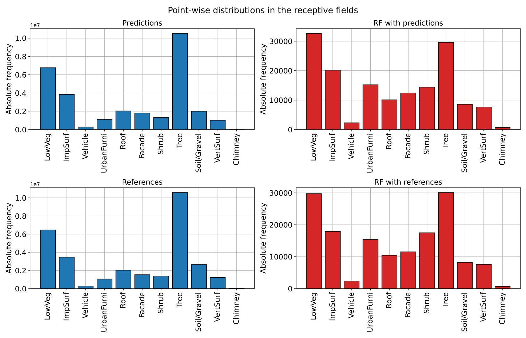
Visualization of the distribution of classes along the receptive fields. Blue for straightforward absolute frequencies, red for counting receptive fields with at least one case of a given class.

Predictive pipeline

The predictive pipeline will use the model trained on the first point cloud to compute an urban semantic segmentation on a validation point cloud. More concretely, the validation point cloud corresponds to the March 2018 epoch of the Hessigheim dataset. The same Standardizer used to standardize the reflectance values of the training point cloud has been used with the validation point cloud. Using the same Standardizer implies considering the mean and standard deviation from the distribution of the training dataset.

The predictions will be exported through the ClassifiedPcloudWriter, which means the boolean mask on success and fail will be available. Also, the ClassificationEvaluator will be used to quantify the quality of the predictions through many evaluation metrics. Uncertainty measurements are also computed through the ClassificationUncertaintyEvaluator.

The JSON below corresponds to the described predictive pipeline.

{
  "in_pcloud": [
    "/mnt/netapp2/Store_uscciaep/lidar_data/hessigheim/vl3d/mined/Mar18_val_hsv_std.laz"
  ],
  "out_pcloud": [
    "/mnt/netapp2/Store_uscciaep/lidar_data/hessigheim/vl3d/kpconv_R/T1/preds/val/*"
  ],
  "sequential_pipeline": [
    {
      "predict": "PredictivePipeline",
      "model_path": "/mnt/netapp2/Store_uscciaep/lidar_data/hessigheim/vl3d/kpconv_R/T1/pipe/KPC_T1.pipe"
    },
    {
        "writer": "ClassifiedPcloudWriter",
        "out_pcloud": "*predicted.las"
    },
    {
      "writer": "PredictionsWriter",
      "out_preds": "*predictions.lbl"
    },
    {
      "eval": "ClassificationEvaluator",
      "class_names": ["LowVeg", "ImpSurf", "Vehicle", "UrbanFurni", "Roof", "Facade", "Shrub", "Tree", "Soil/Gravel", "VertSurf", "Chimney"],
      "metrics": ["OA", "P", "R", "F1", "IoU", "wP", "wR", "wF1", "wIoU", "MCC", "Kappa"],
      "class_metrics": ["P", "R", "F1", "IoU"],
      "report_path": "*report/global_eval.log",
      "class_report_path": "*report/class_eval.log",
      "confusion_matrix_report_path" : "*report/confusion_matrix.log",
      "confusion_matrix_plot_path" : "*plot/confusion_matrix.svg",
      "class_distribution_report_path": "*report/class_distribution.log",
      "class_distribution_plot_path": "*plot/class_distribution.svg"
    },
    {
        "eval": "ClassificationUncertaintyEvaluator",
        "class_names": ["LowVeg", "ImpSurf", "Vehicle", "UrbanFurni", "Roof", "Facade", "Shrub", "Tree", "Soil/Gravel", "VertSurf", "Chimney"],
        "include_probabilities": true,
        "include_weighted_entropy": true,
        "include_clusters": true,
        "weight_by_predictions": false,
        "num_clusters": 10,
        "clustering_max_iters": 128,
        "clustering_batch_size": 1000000,
        "clustering_entropy_weights": false,
        "clustering_reduce_function": "mean",
        "gaussian_kernel_points": 256,
        "report_path": "*uncertainty/uncertainty.las",
        "plot_path": "*uncertainty/"
    }
  ]
}

The table below represents the class-wise evaluation metrics. It shows the precision, recall, F1-score, and intersection over union (IoU) for each class. It can be seen that it is especially problematic to differentiate soil/gravel terrain, as evidenced by its low recall. Besides, roofs are segmented with high recall and precision at the same time. Together with trees, they are clearly the best segmented classes.

CLASS	P	R	F1	IoU
LowVeg	70.550	94.794	80.895	67.918
ImpSurf	90.089	74.809	81.741	69.121
Vehicle	97.718	23.371	37.720	23.244
UrbanFurni	57.470	51.726	54.447	37.407
Roof	94.906	92.246	93.557	87.894
Facade	73.114	83.084	77.781	63.640
Shrub	75.357	40.615	52.782	35.853
Tree	89.740	98.147	93.756	88.245
Soil/Gravel	46.839	4.148	7.620	3.961
VertSurf	83.127	39.119	53.201	36.241
Chimney	83.920	77.021	80.323	67.116

The figure below shows the reference and predicted labels, as well as the fail/success boolean mask representing correctly classified (gray) and misclassified (red) points.

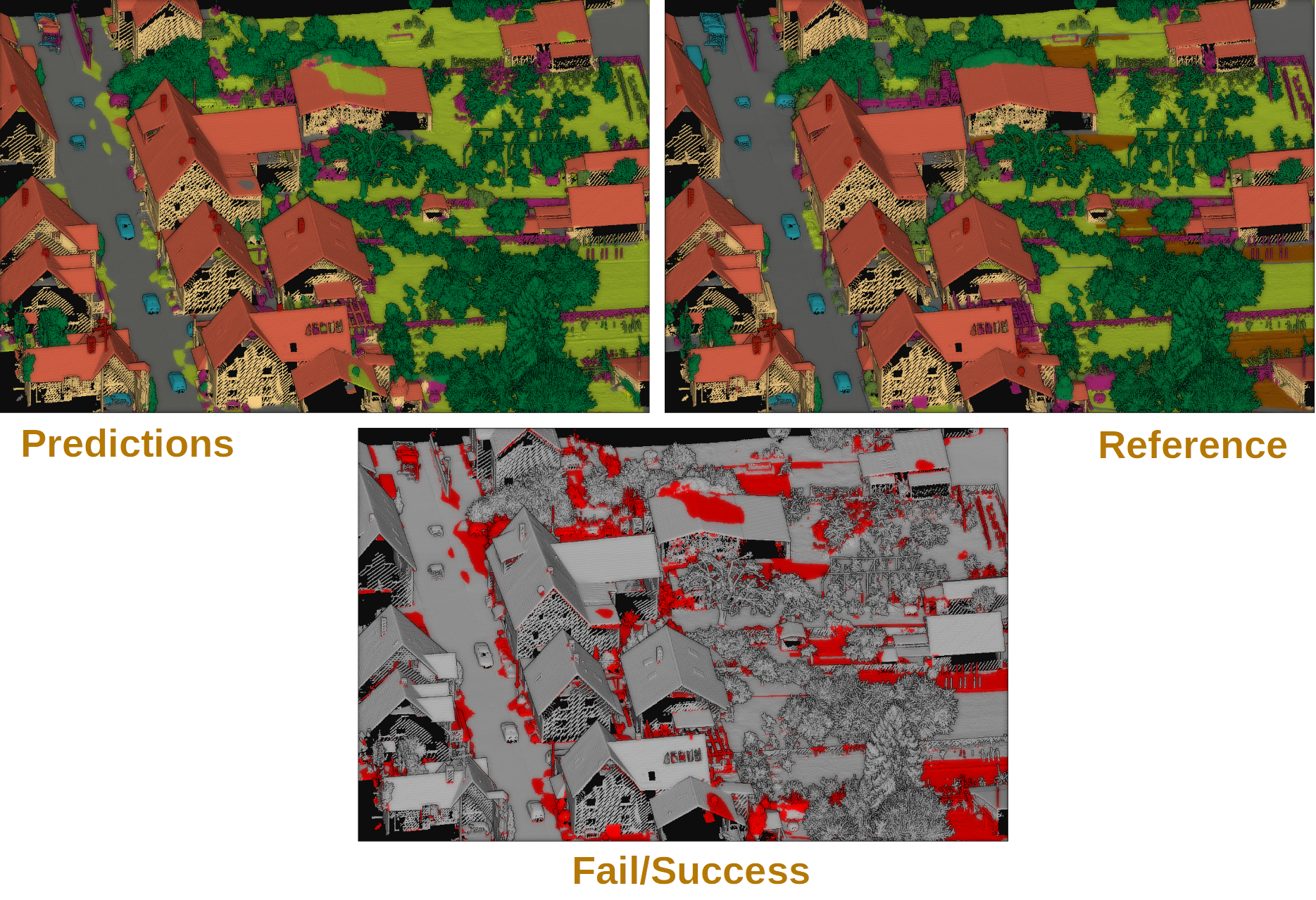
Visualization of the semantic segmentation model applied to previously unseen data. The bottom image shows correctly classified points in gray and misclassified points in red. The predictions and reference images use the same color code for the classes.

SFL-NET-like model

This example shows how to define two different pipelines, one to train a SFL-NET-like model (see SFL-NET documentation) and export it as a PredictivePipeline, the other to use the predictive pipeline to compute a semantic segmentation on a previously unseen point cloud. Readers are referred to the pipelines documentation to read more about how pipelines work and to see more examples.

Training pipeline

The training pipeline will train a ConvAutoencPwiseClassif for the multiclass semantic segmentation of the points. The training point cloud is the “5080_54435” point cloud in the DALES dataset .

The pre-processing strategy computes \(200,000\) receptive fields with \(256\) points at the first depth taken from a spherical neighborhood with a radius of \(6\) meters. It uses an oversampling strategy based on the nearest neighbor to populate receptive fields with not enough points.

The first downsampling (i.e., the one that maps the original input neighborhood to the first receptive field) considers only the nearest neighbor. However, subsequent receptive fields consider \(16\) neighbors when downsampling. The upsampling layers work with the same number of nearest neighbors. The hourglasses are configured with the hyperparameters suggested in the SFL-NET paper (Li et al., 2023) , including the residual hourglass block.

The JSON below corresponds to the described training pipeline.

{
    "in_pcloud": [
        "/oldext4/lidar_data/vl3dhack/data/dales/train/5080_54435.laz"
    ],
    "out_pcloud": [
        "/oldext4/lidar_data/vl3dhack/multiclass/out/DL_SFLNET/T1/*"
    ],
    "sequential_pipeline": [
        {
            "class_transformer": "ClassReducer",
            "on_predictions": false,
            "input_class_names": ["noclass", "ground", "vegetation", "cars", "trucks", "powerlines", "fences", "poles", "buildings"],
            "output_class_names": ["ground", "vegetation", "buildings", "powerlines", "objects", "noclass"],
            "class_groups": [["ground"], ["vegetation"], ["buildings"], ["powerlines"], ["cars", "trucks", "fences", "poles"], ["noclass"]],
            "report_path": "*class_reduction.log",
            "plot_path": "*class_reduction.svg"
        },
        {
            "train": "ConvolutionalAutoencoderPwiseClassifier",
            "training_type": "base",
            "fnames": ["ones"],
            "random_seed": null,
            "model_args": {
                "fnames": ["ones"],
                "num_classes": 6,
                "class_names": ["ground", "vegetation", "buildings", "powerlines", "objects", "noclass"],
                "pre_processing": {
                    "pre_processor": "hierarchical_fps",
                    "support_strategy_num_points": 200000,
                    "to_unit_sphere": false,
                    "support_strategy": "fps",
                    "support_chunk_size": 10000,
                    "support_strategy_fast": true,
                    "receptive_field_oversampling": {
                        "min_points": 2,
                        "strategy": "nearest",
                        "k": 3,
                        "radius": 0.5
                    },
                    "center_on_pcloud": true,
                    "neighborhood": {
                        "type": "sphere",
                        "radius": 6.0,
                        "separation_factor": 0.8
                    },
                    "num_points_per_depth": [256, 128, 64, 32, 16],
                    "fast_flag_per_depth": [false, false, false, false, false],
                    "num_downsampling_neighbors": [1, 16, 16, 16, 16],
                    "num_pwise_neighbors": [16, 16, 16, 16, 16],
                    "num_upsampling_neighbors": [1, 16, 16, 16, 16],
                    "nthreads": -1,
                    "training_receptive_fields_distribution_report_path": "*/training_eval/training_receptive_fields_distribution.log",
                    "training_receptive_fields_distribution_plot_path": "*/training_eval/training_receptive_fields_distribution.svg",
                    "training_receptive_fields_dir": "*/training_eval/training_rf/",
                    "receptive_fields_distribution_report_path": "*/training_eval/receptive_fields_distribution.log",
                    "receptive_fields_distribution_plot_path": "*/training_eval/receptive_fields_distribution.svg",
                    "receptive_fields_dir": "*/training_eval/receptive_fields/",
                    "training_support_points_report_path": "*/training_eval/training_support_points.las",
                    "support_points_report_path": "*/training_eval/support_points.las"
                },
                "feature_extraction": {
                    "type": "LightKPConv",
                    "operations_per_depth": [2, 1, 1, 1, 1],
                    "feature_space_dims": [64, 64, 128, 256, 512, 1024],
                    "bn": true,
                    "bn_momentum": 0.98,
                    "activate": true,
                    "sigma": [6.0, 6.0, 7.5, 9.0, 10.5, 12.0],
                    "kernel_radius": [6.0, 6.0, 6.0, 6.0, 6.0, 6.0],
                    "num_kernel_points": [15, 15, 15, 15, 15, 15],
                    "deformable": [false, false, false, false, false, false],
                    "W_initializer": ["glorot_uniform", "glorot_uniform", "glorot_uniform", "glorot_uniform", "glorot_uniform", "glorot_uniform"],
                    "W_regularizer": [null, null, null, null, null, null],
                    "W_constraint": [null, null, null, null, null, null],
                    "A_trainable": [true, true, true, true, true ,true],
                    "A_regularizer": [null, null, null, null, null, null],
                    "A_constraint": [null, null, null, null, null, null],
                    "A_initializer": ["ones", "ones", "ones", "ones", "ones", "ones"],
                    "hourglass_wrapper": {
                        "internal_dim": [2, 2, 4, 16, 32, 64],
                        "parallel_internal_dim": [8, 8, 16, 32, 64, 128],
                        "activation": ["relu", "relu", "relu", "relu", "relu", "relu"],
                        "activation2": [null, null, null, null, null, null],
                        "regularize": [true, true, true, true, true, true],
                        "W1_initializer": ["glorot_uniform", "glorot_uniform", "glorot_uniform", "glorot_uniform", "glorot_uniform", "glorot_uniform"],
                        "W1_regularizer": [null, null, null, null, null, null],
                        "W1_constraint": [null, null, null, null, null, null],
                        "W2_initializer": ["glorot_uniform", "glorot_uniform", "glorot_uniform", "glorot_uniform", "glorot_uniform", "glorot_uniform"],
                        "W2_regularizer": [null, null, null, null, null, null],
                        "W2_constraint": [null, null, null, null, null, null],
                        "loss_factor": 0.1,
                        "subspace_factor": 0.125,
                        "feature_dim_divisor": 4,
                        "bn": false,
                        "bn_momentum": 0.98,
                        "out_bn": true,
                        "out_bn_momentum": 0.98,
                        "out_activation": "relu"
                    }
                },
                "features_alignment": null,
                "downsampling_filter": "strided_lightkpconv",
                "upsampling_filter": "mean",
                "upsampling_bn": true,
                "upsampling_momentum": 0.98,
                "upsampling_hourglass": {
                    "activation": "relu",
                    "activation2": null,
                    "regularize": true,
                    "W1_initializer": "glorot_uniform",
                    "W1_regularizer": null,
                    "W1_constraint": null,
                    "W2_initializer": "glorot_uniform",
                    "W2_regularizer": null,
                    "W2_constraint": null,
                    "loss_factor": 0.1,
                    "subspace_factor": 0.125
                },
                "conv1d": false,
                "conv1d_kernel_initializer": "glorot_normal",
                "output_kernel_initializer": "glorot_normal",
                "model_handling": {
                    "summary_report_path": "*/model_summary.log",
                    "training_history_dir": "*/training_eval/history",
                    "class_weight": [1.0, 1.0, 1.0, 1.0, 1.0, 0.0],
                    "training_epochs": 300,
                    "batch_size": 64,
                    "training_sequencer": {
                        "type": "DLSequencer",
                        "random_shuffle_indices": true,
                        "augmentor": {
                            "transformations": [
                                    {
                                        "type": "Rotation",
                                        "axis": [0, 0, 1],
                                        "angle_distribution": {
                                            "type": "uniform",
                                            "start": -3.141592,
                                            "end": 3.141592
                                        }
                                    },
                                    {
                                        "type": "Scale",
                                        "scale_distribution": {
                                            "type": "uniform",
                                            "start": 0.99,
                                            "end": 1.01
                                        }
                                    },
                                    {
                                        "type": "Jitter",
                                        "noise_distribution": {
                                            "type": "normal",
                                            "mean": 0,
                                            "stdev": 0.001
                                        }
                                    }
                            ]
                        }
                    },
                    "prediction_reducer": {
                        "reduce_strategy" : {
                            "type": "MeanPredReduceStrategy"
                        },
                        "select_strategy": {
                            "type": "ArgMaxPredSelectStrategy"
                        }
                    },
                    "checkpoint_path": "*/checkpoint.weights.h5",
                    "checkpoint_monitor": "loss",
                    "learning_rate_on_plateau": {
                        "monitor": "loss",
                        "mode": "min",
                        "factor": 0.1,
                        "patience": 2000,
                        "cooldown": 5,
                        "min_delta": 0.01,
                        "min_lr": 1e-6
                    }
                },
                "compilation_args": {
                    "optimizer": {
                        "algorithm": "Adam",
                        "learning_rate": {
                            "schedule": "exponential_decay",
                            "schedule_args": {
                                "initial_learning_rate": 1e-2,
                                "decay_steps": 9000,
                                "decay_rate": 0.96,
                                "staircase": false
                            }
                        }
                    },
                    "loss": {
                        "function": "class_weighted_categorical_crossentropy"
                    },
                    "metrics": [
                        "categorical_accuracy"
                    ]
                },
                "architecture_graph_path": "*/model_graph.png",
                "architecture_graph_args": {
                    "show_shapes": true,
                    "show_dtype": true,
                    "show_layer_names": true,
                    "rankdir": "TB",
                    "expand_nested": true,
                    "dpi": 300,
                    "show_layer_activations": true
                }
            },
            "autoval_metrics": ["OA", "P", "R", "F1", "IoU", "wP", "wR", "wF1", "wIoU", "MCC", "Kappa"],
            "training_evaluation_metrics": ["OA", "P", "R", "F1", "IoU", "wP", "wR", "wF1", "wIoU", "MCC", "Kappa"],
            "training_class_evaluation_metrics": ["P", "R", "F1", "IoU"],
            "training_evaluation_report_path": "*/training_eval/evaluation.log",
            "training_class_evaluation_report_path": "*/training_eval/class_evaluation.log",
            "training_confusion_matrix_report_path": "*/training_eval/confusion.log",
            "training_confusion_matrix_plot_path": "*/training_eval/confusion.svg",
            "training_class_distribution_report_path": "*/training_eval/class_distribution.log",
            "training_class_distribution_plot_path": "*/training_eval/class_distribution.svg",
            "training_classified_point_cloud_path": "*/training_eval/classified_point_cloud.las",
            "training_activations_path": null
        },
        {
            "writer": "PredictivePipelineWriter",
            "out_pipeline": "*/model/SFLNET.pipe",
            "include_writer": false,
            "include_imputer": true,
            "include_feature_transformer": true,
            "include_miner": true,
            "include_class_transformer": false,
            "include_clustering": false,
            "ignore_predictions": false
        }
    ]
}

The figure below represents the \(200,000\) training the support points. The SFL-NET model has been trained on \(200,000\) spherical neighborhoods (with \(6\) meters radius) of \(256\) neighbors each, i.e., a total number of \(51,200,000\) points have been used for training.

Visualization of the \(200,000\) training support points used as the centers of the spherical neighborhoods used during training.

Predictive pipeline

The predictive pipeline will use the model trained on the first point cloud to compute the multiclass semantic segmentation on a validation point cloud. More concretely, the validation point cloud corresponds to the “5145_54470” point cloud of the DALES dataset .

The predictions will be exported through the ClassifiedPcloudWriter, which means the boolean mask on success and fail will be available. Also, the ClassificationEvaluator will be used to quantify the quality of the predictions through many evaluation metrics. Uncertainty measurements are also computed through the ClassificationUncertaintyEvaluator.

The JSON below corresponds to the described predictive pipeline.

{
    "in_pcloud": [
        "/oldext4/lidar_data/vl3dhack/data/dales/test/5145_54470.laz"
    ],
    "out_pcloud": [
        "/oldext4/lidar_data/vl3dhack/multiclass/out/DL_SFLNET/T1/pred/5145_54470/*"
    ],
    "sequential_pipeline": [
        {
            "class_transformer": "ClassReducer",
            "on_predictions": false,
            "input_class_names": ["noclass", "ground", "vegetation", "cars", "trucks", "powerlines", "fences", "poles", "buildings"],
            "output_class_names": ["ground", "vegetation", "buildings", "powerlines", "objects", "noclass"],
            "class_groups": [["ground"], ["vegetation"], ["buildings"], ["powerlines"], ["cars", "trucks", "fences", "poles"], ["noclass"]],
            "report_path": "*class_reduction.log",
            "plot_path": "*class_reduction.svg"
        },
        {
            "predict": "PredictivePipeline",
            "model_path": "/oldext4/lidar_data/vl3dhack/multiclass/out/DL_SFLNET/T1/model/SFLNET.pipe",
            "nn_path": null
        },
        {
            "eval": "ClassificationEvaluator",
            "class_names": ["ground", "vegetation", "buildings", "powerlines", "objects", "noclass"],
            "ignore_classes": ["noclass"],
            "metrics": ["OA", "P", "R", "F1", "IoU", "wP", "wR", "wF1", "wIoU", "MCC", "Kappa"],
            "class_metrics": ["P", "R", "F1", "IoU"],
            "report_path": "*report/global_eval.log",
            "class_report_path": "*report/class_eval.log",
            "confusion_matrix_report_path" : "*/report/confusion_matrix.log",
            "confusion_matrix_plot_path" : "*/report/confusion_matrix.svg",
            "class_distribution_report_path": "*/report/class_distribution.log",
            "class_distribution_plot_path": "*/report/class_distribution.svg"
        },
        {
            "writer": "ClassifiedPcloudWriter",
            "out_pcloud": "*predicted.las"
        }
    ]
}

The table below represents the global evaluation metrics. It shows the overall accuracy (OA), precision (P), recall (R), F1-score (F1), intersection over union (IoU), all of them weighted by the number of points, the Matthew’s correlation coefficient (MCC), and the Cohen’s Kappa score (Kappa).

OA	P	R	F1	IoU	wP	wR	wF1	wIoU	MCC	Kappa
96.739	90.228	89.519	89.806	82.580	96.706	96.739	96.699	93.753	94.850	94.827

The figure below shows the reference and predicted labels, as well as the fail/success boolean mask representing correctly classified (gray) and misclassified (red) points.

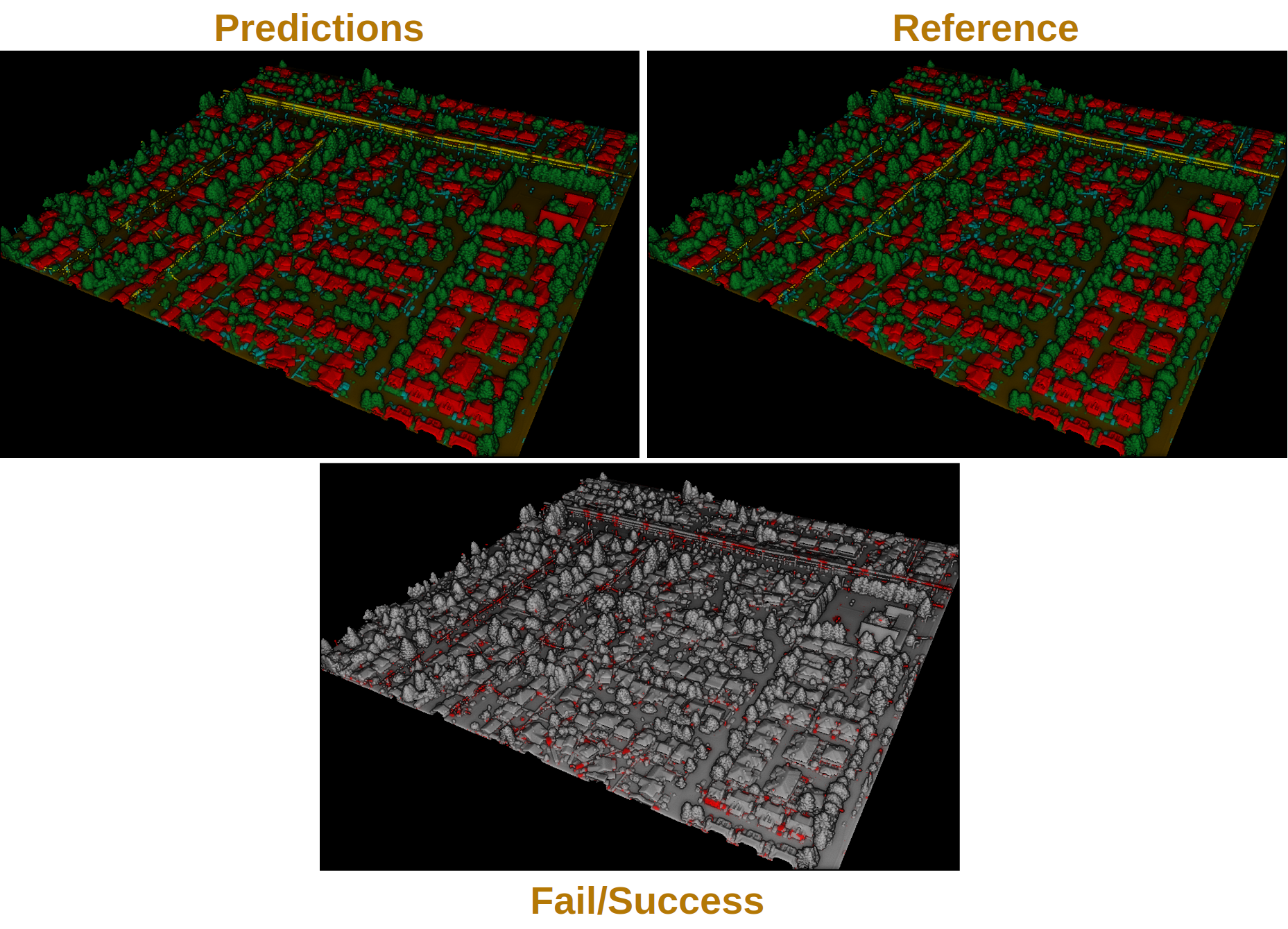
Visualization of the semantic segmentation model applied to previously unseen data. The bottom image shows correctly classified points in gray and misclassified points in red. The predictions and reference images use the same color code for the classes.

PointTransformer-based model

This example shows how to define two different pipelines, one to train a PointTransformer-based model (see PointTransformer documentation) and export it as a PredictivePipeline, the other to use the predictive pipeline to compute a semantic segmentation on a previously unseen point cloud. Readers are referred to the pipelines documentation to read more about how pipelines work and to see more examples.

Training pipeline

The training pipeline will train a ConvAutoencPwiseClassif for the multiclass semantic segmentation of the points. The training point cloud is generated from the March 2018 training point cloud in the Hessigheim dataset by transforming the RGB color components to its HSV representation with HSV from RGB miner.

The pre-processing strategy computes \(25,000\) receptive fields with \(4096\) points at the first depth taken from a spherical neighborhood with a radius of \(5\) meters. It uses an oversampling strategy based on nearest neighbors to populate receptive fields with not enough points.

The first downsampling (i.e., the one that maps the original input neighborhood to the first receptive field) considers the closest neighbor. Subsequent receptive fields consider the mean of the \(16\) closest neighbors when downsampling. The upsampling layers work with the same number of nearest neighbors. Besides, an Hourglass blocks are used both to wrap the main branch and to compute a parallel branch.

The JSON below corresponds to the described training pipeline.

{
    "in_pcloud": [
        "/ext4/hei/Hessigheim_Benchmark/Epoch_March2018/vl3d/mined/Mar18_train_hsv_std.laz"
    ],
    "out_pcloud": [
        "/ext4/hei/Hessigheim_Benchmark/Epoch_March2018/vl3d/out/pttransf/T1/*"
    ],
    "sequential_pipeline": [
        {
            "train": "ConvolutionalAutoencoderPwiseClassifier",
            "training_type": "base",
            "fnames": ["ones", "HSV_Hrad", "HSV_S", "HSV_V"],
            "random_seed": null,
            "model_args": {
                "fnames": ["ones", "HSV_Hrad", "HSV_S", "HSV_V"],
                "num_classes": 11,
                "class_names": ["LowVeg", "ImpSurf", "Vehicle", "UrbanFurni", "Roof", "Facade", "Shrub", "Tree", "Soil/Gravel", "VertSurf", "Chimney"],
                "pre_processing": {
                    "pre_processor": "hierarchical_fpspp",
                    "support_strategy_num_points": 25000,
                    "to_unit_sphere": false,
                    "support_strategy": "fps",
                    "support_strategy_fast": 2,
                    "min_distance": 0.03,
                    "receptive_field_oversampling": {
                        "min_points": 2,
                        "strategy": "nearest",
                        "k": 3,
                        "radius": 0.5
                    },
                    "center_on_pcloud": true,
                    "training_class_distribution": [2250, 2250, 2250, 2250, 2250, 2250, 2250, 2250, 2250, 2250, 2250],
                    "neighborhood": {
                        "type": "sphere",
                        "radius": 5.0,
                        "separation_factor": 0.8
                    },
                    "num_points_per_depth": [4096, 1024, 256, 64, 16],
                    "fast_flag_per_depth": [4, 4, false, false, false],
                    "num_downsampling_neighbors": [1, 16, 16, 16, 16],
                    "num_pwise_neighbors": [16, 16, 16, 16, 16],
                    "num_upsampling_neighbors": [1, 16, 16, 16, 16],
                    "nthreads": -1,
                    "training_receptive_fields_distribution_report_path": null,
                    "training_receptive_fields_distribution_plot_path": null,
                    "training_receptive_fields_dir": null,
                    "receptive_fields_distribution_report_path": null,
                    "receptive_fields_distribution_plot_path": null,
                    "receptive_fields_dir": null,
                    "training_support_points_report_path": null,
                    "support_points_report_path": null
                },
                "feature_extraction": {
                    "type": "PointTransformer",
                    "operations_per_depth": [2, 1, 1, 1, 1],
                    "feature_space_dims": [64, 64, 96, 128, 192, 256],
                    "bn": false,
                    "bn_momentum": 0.98,
                    "activate": false,
                    "Phi_initializer": ["glorot_uniform", "glorot_uniform", "glorot_uniform", "glorot_uniform", "glorot_uniform", "glorot_uniform"],
                    "Phi_regularizer": [null, null, null, null, null, null],
                    "Phi_constraint": [null, null, null, null, null, null],
                    "Psi_initializer": ["glorot_uniform", "glorot_uniform", "glorot_uniform", "glorot_uniform", "glorot_uniform", "glorot_uniform"],
                    "Psi_regularizer": [null, null, null, null, null, null],
                    "Psi_constraint": [null, null, null, null, null, null],
                    "A_initializer": ["glorot_uniform", "glorot_uniform", "glorot_uniform", "glorot_uniform", "glorot_uniform", "glorot_uniform"],
                    "A_regularizer": [null, null, null, null, null, null],
                    "A_constraint": [null, null, null, null, null, null],
                    "Gamma_initializer": ["glorot_uniform", "glorot_uniform", "glorot_uniform", "glorot_uniform", "glorot_uniform", "glorot_uniform"],
                    "Gamma_regularizer": [null, null, null, null, null, null],
                    "Gamma_constraint": [null, null, null, null, null, null],
                    "Theta_initializer": ["glorot_uniform", "glorot_uniform", "glorot_uniform", "glorot_uniform", "glorot_uniform", "glorot_uniform"],
                    "Theta_regularizer": [null, null, null, null, null, null],
                    "Theta_constraint": [null, null, null, null, null, null],
                    "ThetaTilde_initializer": ["glorot_uniform", "glorot_uniform", "glorot_uniform", "glorot_uniform", "glorot_uniform", "glorot_uniform"],
                    "ThetaTilde_regularizer": [null, null, null, null, null, null],
                    "ThetaTilde_constraint": [null, null, null, null, null, null],
                    "phi_initializer": ["glorot_uniform", "glorot_uniform", "glorot_uniform", "glorot_uniform", "glorot_uniform", "glorot_uniform"],
                    "phi_regularizer": [null, null, null, null, null, null],
                    "phi_constraint": [null, null, null, null, null, null],
                    "psi_initializer": ["glorot_uniform", "glorot_uniform", "glorot_uniform", "glorot_uniform", "glorot_uniform", "glorot_uniform"],
                    "psi_regularizer": [null, null, null, null, null, null],
                    "psi_constraint": [null, null, null, null, null, null],
                    "a_initializer": ["glorot_uniform", "glorot_uniform", "glorot_uniform", "glorot_uniform", "glorot_uniform", "glorot_uniform"],
                    "a_regularizer": [null, null, null, null, null, null],
                    "a_constraint": [null, null, null, null, null, null],
                    "gamma_initializer": ["glorot_uniform", "glorot_uniform", "glorot_uniform", "glorot_uniform", "glorot_uniform", "glorot_uniform"],
                    "gamma_regularizer": [null, null, null, null, null, null],
                    "gamma_constraint": [null, null, null, null, null, null],
                    "theta_initializer": ["glorot_uniform", "glorot_uniform", "glorot_uniform", "glorot_uniform", "glorot_uniform", "glorot_uniform"],
                    "theta_regularizer": [null, null, null, null, null, null],
                    "theta_constraint": [null, null, null, null, null, null],
                    "thetaTilde_initializer": ["glorot_uniform", "glorot_uniform", "glorot_uniform", "glorot_uniform", "glorot_uniform", "glorot_uniform"],
                    "thetaTilde_regularizer": [null, null, null, null, null, null],
                    "thetaTilde_constraint": [null, null, null, null, null, null],
                    "hourglass_wrapper": {
                        "internal_dim": [2, 2, 4, 16, 32, 64],
                        "parallel_internal_dim": [8, 8, 16, 32, 64, 128],
                        "activation": ["relu", "relu", "relu", "relu", "relu", "relu"],
                        "activation2": [null, null, null, null, null, null],
                        "activate_postwrap": true,
                        "activate_residual": false,
                        "regularize": [true, true, true, true, true, true],
                        "W1_initializer": ["glorot_uniform", "glorot_uniform", "glorot_uniform", "glorot_uniform", "glorot_uniform", "glorot_uniform"],
                        "W1_regularizer": [null, null, null, null, null, null],
                        "W1_constraint": [null, null, null, null, null, null],
                        "W2_initializer": ["glorot_uniform", "glorot_uniform", "glorot_uniform", "glorot_uniform", "glorot_uniform", "glorot_uniform"],
                        "W2_regularizer": [null, null, null, null, null, null],
                        "W2_constraint": [null, null, null, null, null, null],
                        "loss_factor": 0.1,
                        "subspace_factor": 0.125,
                        "feature_dim_divisor": 4,
                        "bn": false,
                        "merge_bn": false,
                        "bn_momentum": 0.98,
                        "out_bn": true,
                        "out_bn_momentum": 0.98,
                        "out_activation": "relu"
                    }
                },
                "features_alignment": null,
                "downsampling_filter": "mean",
                "upsampling_filter": "mean",
                "upsampling_bn": true,
                "upsampling_momentum": 0.98,
                "conv1d": false,
                "conv1d_kernel_initializer": "glorot_normal",
                "output_kernel_initializer": "glorot_normal",
                "model_handling": {
                    "summary_report_path": "*/model_summary.log",
                    "training_history_dir": "*/training_eval/history",
                    "class_weight": [1.0, 1.0, 1.0, 1.0, 1.0, 1.0, 1.0, 1.0, 1.0, 1.0, 1.0],
                    "training_epochs": 200,
                    "batch_size": 32,
                    "training_sequencer": {
                        "type": "DLSequencer",
                        "random_shuffle_indices": true,
                        "augmentor": {
                            "transformations": [
                                    {
                                        "type": "Rotation",
                                        "axis": [0, 0, 1],
                                        "angle_distribution": {
                                            "type": "uniform",
                                            "start": -3.141592,
                                            "end": 3.141592
                                        }
                                    },
                                    {
                                        "type": "Scale",
                                        "scale_distribution": {
                                            "type": "uniform",
                                            "start": 0.985,
                                            "end": 1.015
                                        }
                                    },
                                    {
                                        "type": "Jitter",
                                        "noise_distribution": {
                                            "type": "normal",
                                            "mean": 0,
                                            "stdev": 0.0033
                                        }
                                    }
                            ]
                        }
                    },
                    "prediction_reducer": {
                        "reduce_strategy" : {
                            "type": "MeanPredReduceStrategy"
                        },
                        "select_strategy": {
                            "type": "ArgMaxPredSelectStrategy"
                        }
                    },
                    "checkpoint_path": "*/checkpoint.weights.h5",
                    "checkpoint_monitor": "loss",
                    "learning_rate_on_plateau": {
                        "monitor": "loss",
                        "mode": "min",
                        "factor": 0.1,
                        "patience": 2000,
                        "cooldown": 5,
                        "min_delta": 0.01,
                        "min_lr": 1e-6
                    }
                },
                "compilation_args": {
                    "optimizer": {
                        "algorithm": "Adam",
                        "learning_rate": {
                            "schedule": "exponential_decay",
                            "schedule_args": {
                                "initial_learning_rate": 1e-2,
                                "decay_steps": 1000,
                                "decay_rate": 0.96,
                                "staircase": false
                            }
                        }
                    },
                    "loss": {
                        "function": "class_weighted_categorical_crossentropy"
                    },
                    "metrics": [
                        "categorical_accuracy"
                    ]
                },
                "architecture_graph_path": "*/model_graph.png",
                "architecture_graph_args": {
                    "show_shapes": true,
                    "show_dtype": true,
                    "show_layer_names": true,
                    "rankdir": "TB",
                    "expand_nested": true,
                    "dpi": 300,
                    "show_layer_activations": true
                }
            },
            "autoval_metrics": null,
            "training_evaluation_metrics": null,
            "training_class_evaluation_metrics": null,
            "training_evaluation_report_path": null,
            "training_class_evaluation_report_path": null,
            "training_confusion_matrix_report_path": null,
            "training_confusion_matrix_plot_path": null,
            "training_class_distribution_report_path": null,
            "training_class_distribution_plot_path": null,
            "training_classified_point_cloud_path": null,
            "training_activations_path": null
        },
        {
            "writer": "PredictivePipelineWriter",
            "out_pipeline": "*/model/PointTransformer.pipe",
            "include_writer": false,
            "include_imputer": false,
            "include_feature_transformer": false,
            "include_miner": false,
            "include_class_transformer": false,
            "include_clustering": false,
            "ignore_predictions": false
        }
    ]
}

The figure below represents the evolution among the many training epochs of the categorical accuracy, the categorical cross-entropy loss, and the learning rate.

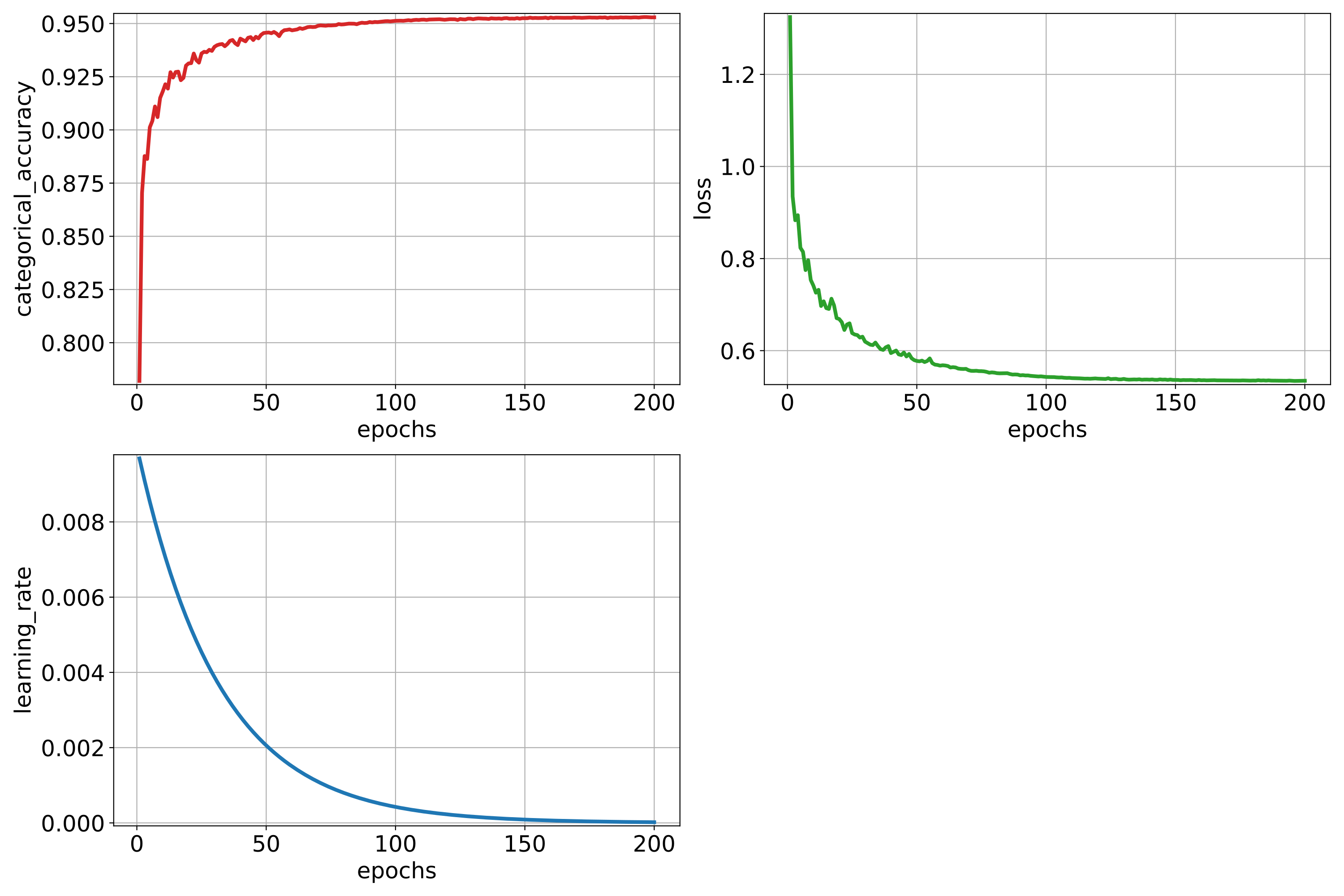
Visualization of the categorical accuracy, the categorical cross-entropy loss, and the learning rate among \(200\) epochs.

Predictive pipeline

The predictive pipeline will use the model on a validation point cloud from the same dataset and epoch. The predictions will be evaluated through ClassificationEvaluator and they will be exported together with their uncertainties through ClassificationUncertaintyEvaluator.

The JSON below corresponds to the described predictive pipeline.

{
  "in_pcloud": [
    "/ext4/hei/Hessigheim_Benchmark/Epoch_March2018/vl3d/mined/Mar18_val_hsv_std.laz"
  ],
  "out_pcloud": [
    "/ext4/hei/Hessigheim_Benchmark/Epoch_March2018/vl3d/out/pttransf/T1/preds/*"
  ],
  "sequential_pipeline": [
    {
      "predict": "PredictivePipeline",
      "model_path": "/ext4/hei/Hessigheim_Benchmark/Epoch_March2018/vl3d/out/pttransf/T1/model/PointTransformer.pipe"
    },
    {
      "eval": "ClassificationEvaluator",
      "class_names": ["LowVeg", "ImpSurf", "Vehicle", "UrbanFurni", "Roof", "Facade", "Shrub", "Tree", "Soil/Gravel", "VertSurf", "Chimney"],
      "metrics": ["OA", "P", "R", "F1", "IoU", "wP", "wR", "wF1", "wIoU", "MCC", "Kappa"],
      "class_metrics": ["P", "R", "F1", "IoU"],
      "report_path": "*report/global_eval.log",
      "class_report_path": "*report/class_eval.log",
      "confusion_matrix_report_path" : "*report/confusion_matrix.log",
      "confusion_matrix_plot_path" : "*plot/confusion_matrix.svg",
      "class_distribution_report_path": "*report/class_distribution.log",
      "class_distribution_plot_path": "*plot/class_distribution.svg"
    },
    {
        "eval": "ClassificationUncertaintyEvaluator",
        "class_names": ["LowVeg", "ImpSurf", "Vehicle", "UrbanFurni", "Roof", "Facade", "Shrub", "Tree", "Soil/Gravel", "VertSurf", "Chimney"],
        "include_probabilities": true,
        "include_weighted_entropy": false,
        "include_clusters": false,
        "weight_by_predictions": false,
        "num_clusters": 0,
        "clustering_max_iters": 0,
        "clustering_batch_size": 0,
        "clustering_entropy_weights": false,
        "clustering_reduce_function": null,
        "gaussian_kernel_points": 0,
        "report_path": "*uncertainty/uncertainty.las",
        "plot_path": "*uncertainty/"
    }
  ]
}

The table below represents the global evaluation metrics. It shows the overall accuracy (OA), precision (P), recall (R), F1-score (F1), intersection over union (IoU), all of them weighted by the number of points, the Matthew’s correlation coefficient (MCC), and the Cohen’s Kappa score (Kappa).

OA	P	R	F1	IoU	wP	wR	wF1	wIoU	MCC	Kappa
87.721	81.267	70.418	74.237	62.021	86.984	87.721	86.813	78.751	84.803	84.715

The figure below shows the reference and predicted labels, the class ambiguity as a point-wise uncertainty measurement, and the binary error mask (gray for correctly classified points, red for misclassified ones).

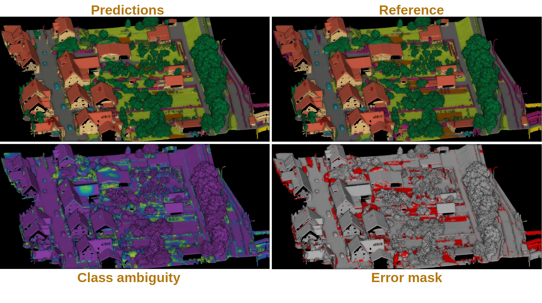
Visualization of the semantic segmentation model applied to previously unseen data. The bottom-right image shows correctly classified points in gray and misclassified points in red. The predictions and reference images use the same color code for the classes. The class ambiguity is represented with purple color for low-uncertainty regions and yellow for high-uncertainty ones.

GroupedPointTransformer-based model

This example shows how to define two different pipelines, one to train a GroupedPointTransformer-based model (see GroupedPointTransformer documentation) and export it as a PredictivePipeline, the other to use the predictive pipeline to compute a semantic segmentation on a previously unseen point cloud. Readers are referred to the pipelines documentation to read more about how pipelines work and to see more examples.

Training pipeline

The training pipeline will train a ConvAutoencPwiseClassif for the multiclass semantic segmentation of the points. The training point cloud is generated from the March 2018 training point cloud in the Hessigheim dataset by transforming the RGB color components to its HSV representation with HSV from RGB miner.

The pre-processing strategy computes \(25,000\) receptive fields with \(4096\) points at the first depth taken from a spherical neighborhood with a radius of \(5\) meters. It uses an oversampling strategy based on nearest neighbors to populate receptive fields with not enough points.

The first downsampling (i.e., the one that maps the original input neighborhood to the first receptive field) considers the closest neighbor. Subsequent receptive fields consider the mean of the \(16\) closest neighbors when downsampling. The upsampling layers work with the same number of nearest neighbors.

The JSON below corresponds to the described training pipeline.

{
    "in_pcloud": [
        "/ext4/hei/Hessigheim_Benchmark/Epoch_March2018/vl3d/mined/Mar18_train_hsv_std.laz"
    ],
    "out_pcloud": [
        "/ext4/hei/Hessigheim_Benchmark/Epoch_March2018/vl3d/out/gpttransf/T1/*"
    ],
    "sequential_pipeline": [
        {
            "train": "ConvolutionalAutoencoderPwiseClassifier",
            "training_type": "base",
            "fnames": ["ones", "HSV_Hrad", "HSV_S", "HSV_V"],
            "random_seed": null,
            "model_args": {
                "fnames": ["ones", "HSV_Hrad", "HSV_S", "HSV_V"],
                "num_classes": 11,
                "class_names": ["LowVeg", "ImpSurf", "Vehicle", "UrbanFurni", "Roof", "Facade", "Shrub", "Tree", "Soil/Gravel", "VertSurf", "Chimney"],
                "pre_processing": {
                    "pre_processor": "hierarchical_fpspp",
                    "support_strategy_num_points": 25000,
                    "to_unit_sphere": false,
                    "support_strategy": "fps",
                    "support_strategy_fast": 2,
                    "min_distance": 0.03,
                    "receptive_field_oversampling": {
                        "min_points": 2,
                        "strategy": "nearest",
                        "k": 3,
                        "radius": 0.5
                    },
                    "center_on_pcloud": true,
                    "training_class_distribution": [2250, 2250, 2250, 2250, 2250, 2250, 2250, 2250, 2250, 2250, 2250],
                    "neighborhood": {
                        "type": "sphere",
                        "radius": 5.0,
                        "separation_factor": 0.8
                    },
                    "num_points_per_depth": [4096, 1024, 256, 64, 16],
                    "fast_flag_per_depth": [4, 4, false, false, false],
                    "num_downsampling_neighbors": [1, 16, 16, 16, 16],
                    "num_pwise_neighbors": [16, 16, 16, 16, 16],
                    "num_upsampling_neighbors": [1, 16, 16, 16, 16],
                    "nthreads": -1,
                    "training_receptive_fields_distribution_report_path": null,
                    "training_receptive_fields_distribution_plot_path": null,
                    "training_receptive_fields_dir": null,
                    "receptive_fields_distribution_report_path": null,
                    "receptive_fields_distribution_plot_path": null,
                    "receptive_fields_dir": null,
                    "training_support_points_report_path": null,
                    "support_points_report_path": null
                },
                "feature_extraction": {
                    "type": "GroupedPointTransformer",
                    "operations_per_depth": [2, 1, 1, 1, 1],
                    "feature_space_dims": [64, 64, 96, 128, 192, 256],
                    "init_ftransf_bn": true,
                    "init_ftransf_bn_momentum": 0.98,
                    "groups": [8, 8, 12, 16, 24, 32],
                    "dropout_rate": [0.25, 0.25, 0.25, 0.25, 0.25, 0.25],
                    "bn": false,
                    "bn_momentum": 0.98,
                    "activate": false,
                    "Q_initializer": ["glorot_uniform", "glorot_uniform", "glorot_uniform", "glorot_uniform", "glorot_uniform", "glorot_uniform"],
                    "Q_regularizer": [null, null, null, null, null, null],
                    "Q_constraint": [null, null, null, null, null, null],
                    "Q_bn_momentum": [0.98, 0.98, 0.98, 0.98, 0.98, 0.98],
                    "q_initializer": ["glorot_uniform", "glorot_uniform", "glorot_uniform", "glorot_uniform", "glorot_uniform", "glorot_uniform"],
                    "q_regularizer": [null, null, null, null, null, null],
                    "q_constraint": [null, null, null, null, null, null],
                    "K_initializer": ["glorot_uniform", "glorot_uniform", "glorot_uniform", "glorot_uniform", "glorot_uniform", "glorot_uniform"],
                    "K_regularizer": [null, null, null, null, null, null],
                    "K_constraint": [null, null, null, null, null, null],
                    "K_bn_momentum": [0.98, 0.98, 0.98, 0.98, 0.98, 0.98],
                    "k_initializer": ["glorot_uniform", "glorot_uniform", "glorot_uniform", "glorot_uniform", "glorot_uniform", "glorot_uniform"],
                    "k_regularizer": [null, null, null, null, null, null],
                    "k_constraint": [null, null, null, null, null, null],
                    "V_initializer": ["glorot_uniform", "glorot_uniform", "glorot_uniform", "glorot_uniform", "glorot_uniform", "glorot_uniform"],
                    "V_regularizer": [null, null, null, null, null, null],
                    "V_constraint": [null, null, null, null, null, null],
                    "v_initializer": ["glorot_uniform", "glorot_uniform", "glorot_uniform", "glorot_uniform", "glorot_uniform", "glorot_uniform"],
                    "v_regularizer": [null, null, null, null, null, null],
                    "v_constraint": [null, null, null, null, null, null],
                    "ThetaA_initializer": ["glorot_uniform", "glorot_uniform", "glorot_uniform", "glorot_uniform", "glorot_uniform", "glorot_uniform"],
                    "ThetaA_regularizer": [null, null, null, null, null, null],
                    "ThetaA_constraint": [null, null, null, null, null, null],
                    "thetaA_initializer": ["glorot_uniform", "glorot_uniform", "glorot_uniform", "glorot_uniform", "glorot_uniform", "glorot_uniform"],
                    "thetaA_regularizer": [null, null, null, null, null, null],
                    "thetaA_constraint": [null, null, null, null, null, null],
                    "ThetaTildeA_initializer": ["glorot_uniform", "glorot_uniform", "glorot_uniform", "glorot_uniform", "glorot_uniform", "glorot_uniform"],
                    "ThetaTildeA_regularizer": [null, null, null, null, null, null],
                    "ThetaTildeA_constraint": [null, null, null, null, null, null],
                    "thetaTildeA_initializer": ["glorot_uniform", "glorot_uniform", "glorot_uniform", "glorot_uniform", "glorot_uniform", "glorot_uniform"],
                    "thetaTildeA_regularizer": [null, null, null, null, null, null],
                    "thetaTildeA_constraint": [null, null, null, null, null, null],
                    "deltaA_bn_momentum": [0.98, 0.98, 0.98, 0.98, 0.98, 0.98],
                    "ThetaB_initializer": ["glorot_uniform", "glorot_uniform", "glorot_uniform", "glorot_uniform", "glorot_uniform", "glorot_uniform"],
                    "ThetaB_regularizer": [null, null, null, null, null, null],
                    "ThetaB_constraint": [null, null, null, null, null, null],
                    "thetaB_initializer": ["glorot_uniform", "glorot_uniform", "glorot_uniform", "glorot_uniform", "glorot_uniform", "glorot_uniform"],
                    "thetaB_regularizer": [null, null, null, null, null, null],
                    "thetaB_constraint": [null, null, null, null, null, null],
                    "ThetaTildeB_initializer": ["glorot_uniform", "glorot_uniform", "glorot_uniform", "glorot_uniform", "glorot_uniform", "glorot_uniform"],
                    "ThetaTildeB_regularizer": [null, null, null, null, null, null],
                    "ThetaTildeB_constraint": [null, null, null, null, null, null],
                    "thetaTildeB_initializer": ["glorot_uniform", "glorot_uniform", "glorot_uniform", "glorot_uniform", "glorot_uniform", "glorot_uniform"],
                    "thetaTildeB_regularizer": [null, null, null, null, null, null],
                    "thetaTildeB_constraint": [null, null, null, null, null, null],
                    "deltaB_bn_momentum": [0.98, 0.98, 0.98, 0.98, 0.98, 0.98],
                    "Omega_initializer": ["glorot_uniform", "glorot_uniform", "glorot_uniform", "glorot_uniform", "glorot_uniform", "glorot_uniform"],
                    "Omega_regularizer": [null, null, null, null, null, null],
                    "Omega_constraint": [null, null, null, null, null, null],
                    "omega_initializer": ["glorot_uniform", "glorot_uniform", "glorot_uniform", "glorot_uniform", "glorot_uniform", "glorot_uniform"],
                    "omega_regularizer": [null, null, null, null, null, null],
                    "omega_constraint": [null, null, null, null, null, null],
                    "omega_bn_momentum": [0.98, 0.98, 0.98, 0.98, 0.98, 0.98],
                    "OmegaTilde_initializer": ["glorot_uniform", "glorot_uniform", "glorot_uniform", "glorot_uniform", "glorot_uniform", "glorot_uniform"],
                    "OmegaTilde_regularizer": [null, null, null, null, null, null],
                    "OmegaTilde_constraint": [null, null, null, null, null, null],
                    "omegaTilde_initializer": ["glorot_uniform", "glorot_uniform", "glorot_uniform", "glorot_uniform", "glorot_uniform", "glorot_uniform"],
                    "omegaTilde_regularizer": [null, null, null, null, null, null],
                    "omegaTilde_constraint": [null, null, null, null, null, null]
                },
                "features_alignment": null,
                "downsampling_filter": "mean",
                "upsampling_filter": "mean",
                "upsampling_bn": true,
                "upsampling_momentum": 0.98,
                "conv1d": false,
                "conv1d_kernel_initializer": "glorot_normal",
                "output_kernel_initializer": "glorot_normal",
                "model_handling": {
                    "summary_report_path": "*/model_summary.log",
                    "training_history_dir": "*/training_eval/history",
                    "class_weight": [1.0, 1.0, 1.0, 1.0, 1.0, 1.0, 1.0, 1.0, 1.0, 1.0, 1.0],
                    "training_epochs": 200,
                    "batch_size": 32,
                    "training_sequencer": {
                        "type": "DLSequencer",
                        "random_shuffle_indices": true,
                        "augmentor": {
                            "transformations": [
                                    {
                                        "type": "Rotation",
                                        "axis": [0, 0, 1],
                                        "angle_distribution": {
                                            "type": "uniform",
                                            "start": -3.141592,
                                            "end": 3.141592
                                        }
                                    },
                                    {
                                        "type": "Scale",
                                        "scale_distribution": {
                                            "type": "uniform",
                                            "start": 0.985,
                                            "end": 1.015
                                        }
                                    },
                                    {
                                        "type": "Jitter",
                                        "noise_distribution": {
                                            "type": "normal",
                                            "mean": 0,
                                            "stdev": 0.0033
                                        }
                                    }
                            ]
                        }
                    },
                    "prediction_reducer": {
                        "reduce_strategy" : {
                            "type": "MeanPredReduceStrategy"
                        },
                        "select_strategy": {
                            "type": "ArgMaxPredSelectStrategy"
                        }
                    },
                    "checkpoint_path": "*/checkpoint.weights.h5",
                    "checkpoint_monitor": "loss",
                    "learning_rate_on_plateau": {
                        "monitor": "loss",
                        "mode": "min",
                        "factor": 0.1,
                        "patience": 2000,
                        "cooldown": 5,
                        "min_delta": 0.01,
                        "min_lr": 1e-6
                    }
                },
                "compilation_args": {
                    "optimizer": {
                        "algorithm": "Adam",
                        "learning_rate": {
                            "schedule": "exponential_decay",
                            "schedule_args": {
                                "initial_learning_rate": 1e-2,
                                "decay_steps": 1000,
                                "decay_rate": 0.96,
                                "staircase": false
                            }
                        }
                    },
                    "loss": {
                        "function": "class_weighted_categorical_crossentropy"
                    },
                    "metrics": [
                        "categorical_accuracy"
                    ]
                },
                "architecture_graph_path": "*/model_graph.png",
                "architecture_graph_args": {
                    "show_shapes": true,
                    "show_dtype": true,
                    "show_layer_names": true,
                    "rankdir": "TB",
                    "expand_nested": true,
                    "dpi": 300,
                    "show_layer_activations": true
                }
            },
            "autoval_metrics": null,
            "training_evaluation_metrics": null,
            "training_class_evaluation_metrics": null,
            "training_evaluation_report_path": null,
            "training_class_evaluation_report_path": null,
            "training_confusion_matrix_report_path": null,
            "training_confusion_matrix_plot_path": null,
            "training_class_distribution_report_path": null,
            "training_class_distribution_plot_path": null,
            "training_classified_point_cloud_path": null,
            "training_activations_path": null
        },
        {
            "writer": "PredictivePipelineWriter",
            "out_pipeline": "*/model/PointTransformer.pipe",
            "include_writer": false,
            "include_imputer": true,
            "include_feature_transformer": true,
            "include_miner": true,
            "include_class_transformer": false,
            "include_clustering": false,
            "ignore_predictions": false
        }
    ]
}

The figure below represents the evolution among the many training epochs of the categorical accuracy, the categorical cross-entropy loss, and the learning rate.

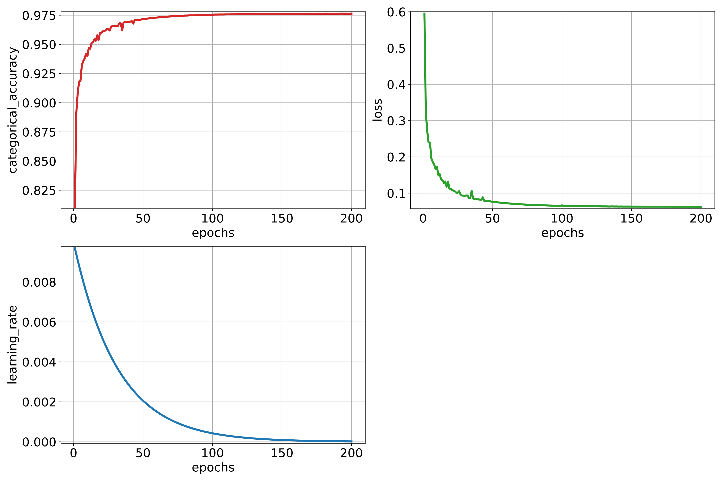
Visualization of the categorical accuracy, the categorical cross-entropy loss, and the learning rate among \(200\) epochs.

Predictive pipeline

The predictive pipeline will use the model on a validation point cloud from the same dataset and epoch. The predictions will be evaluated through ClassificationEvaluator and they will be exported together with their uncertainties through ClassificationUncertaintyEvaluator.

The JSON below corresponds to the described predictive pipeline.

{
  "in_pcloud": [
    "/ext4/hei/Hessigheim_Benchmark/Epoch_March2018/vl3d/mined/Mar18_val_hsv_std.laz"
  ],
  "out_pcloud": [
    "/ext4/hei/Hessigheim_Benchmark/Epoch_March2018/vl3d/out/gpttransf/T1/preds/*"
  ],
  "sequential_pipeline": [
    {
      "predict": "PredictivePipeline",
      "model_path": "/ext4/hei/Hessigheim_Benchmark/Epoch_March2018/vl3d/out/gpttransf/T1/model/PointTransformer.pipe"
    },
    {
      "eval": "ClassificationEvaluator",
      "class_names": ["LowVeg", "ImpSurf", "Vehicle", "UrbanFurni", "Roof", "Facade", "Shrub", "Tree", "Soil/Gravel", "VertSurf", "Chimney"],
      "metrics": ["OA", "P", "R", "F1", "IoU", "wP", "wR", "wF1", "wIoU", "MCC", "Kappa"],
      "class_metrics": ["P", "R", "F1", "IoU"],
      "report_path": "*report/global_eval.log",
      "class_report_path": "*report/class_eval.log",
      "confusion_matrix_report_path" : "*report/confusion_matrix.log",
      "confusion_matrix_plot_path" : "*plot/confusion_matrix.svg",
      "class_distribution_report_path": "*report/class_distribution.log",
      "class_distribution_plot_path": "*plot/class_distribution.svg"
    },
    {
        "eval": "ClassificationUncertaintyEvaluator",
        "class_names": ["LowVeg", "ImpSurf", "Vehicle", "UrbanFurni", "Roof", "Facade", "Shrub", "Tree", "Soil/Gravel", "VertSurf", "Chimney"],
        "include_probabilities": true,
        "include_weighted_entropy": false,
        "include_clusters": false,
        "weight_by_predictions": false,
        "num_clusters": 0,
        "clustering_max_iters": 0,
        "clustering_batch_size": 0,
        "clustering_entropy_weights": false,
        "clustering_reduce_function": null,
        "gaussian_kernel_points": 0,
        "report_path": "*uncertainty/uncertainty.las",
        "plot_path": "*uncertainty/"
    }
  ]
}

The table below represents the global evaluation metrics. It shows the overall accuracy (OA), precision (P), recall (R), F1-score (F1), intersection over union (IoU), all of them weighted by the number of points, the Matthew’s correlation coefficient (MCC), and the Cohen’s Kappa score (Kappa).

OA	P	R	F1	IoU	wP	wR	wF1	wIoU	MCC	Kappa
88.321	81.272	72.783	76.021	64.319	87.675	88.321	87.674	79.734	85.532	85.475

The figure below shows the reference and predicted labels, the class ambiguity as a point-wise uncertainty measurement, and the binary error mask (gray for correctly classified points, red for misclassified ones).

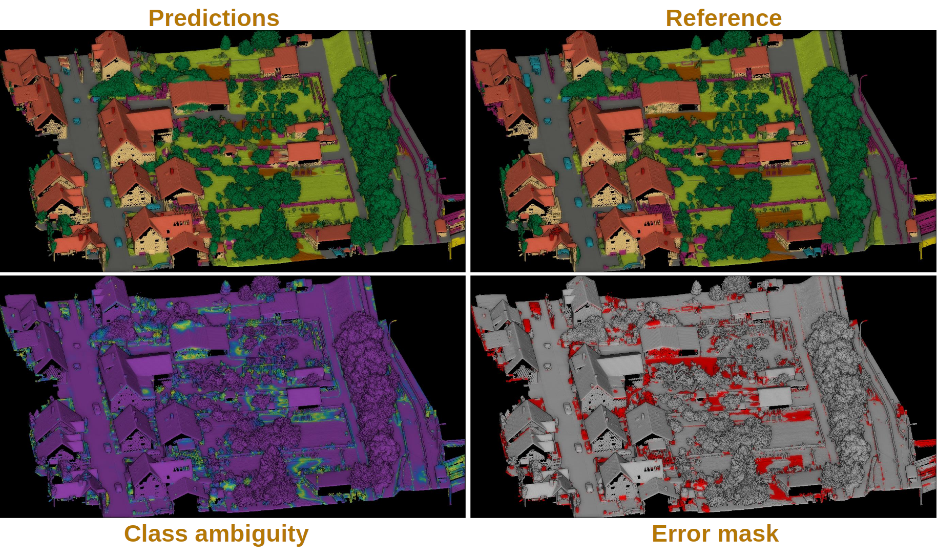
Visualization of the semantic segmentation model applied to previously unseen data. The bottom-right image shows correctly classified points in gray and misclassified points in red. The predictions and reference images use the same color code for the classes. The class ambiguity is represented with purple color for low-uncertainty regions and yellow for high-uncertainty ones.

PointMLP-based model

This example shows how to define two different pipelines, one to train a PointMLP-based model (see Hierarchical PointMLP documentation) and export it as a PredictivePipeline, the other to use the predictive pipeline to compute a semantic segmentation on a previously unseen point cloud. Readers are referred to the pipelines documentation to read more about how pipelines work and to see more examples.

Training pipeline

The training pipeline will train a ConvAutoencPwiseClassif for the multiclass semantic segmentation of the points. The training point cloud is generated from the March 2018 training point cloud in the Hessigheim dataset by transforming the RGB color components to its HSV representation with HSV from RGB miner.

The pre-processing strategy computes \(25,000\) receptive fields with \(4096\) points at the first depth taken from a spherical neighborhood with a radius of \(5\) meters. It uses an oversampling strategy based on nearest neighbors to puplate receptive fields with not enough points.

The first downsampling (i.e., the one that maps the original input neighborhood to the first receptive field) considers the closest neighbor. Subsequent receptive fields consider the mean of the \(16\) closest neighbors when downsampling. The upsampling layers work with the same number of nearest neighbors.

The JSON below corresponds to the described training pipeline.

{
    "in_pcloud": [
        "/ext4/hei/Hessigheim_Benchmark/Epoch_March2018/vl3d/mined/Mar18_train_hsv_std.laz"
    ],
    "out_pcloud": [
        "/ext4/hei/Hessigheim_Benchmark/Epoch_March2018/vl3d/out/pointmlp_dumean_neck_multictxhead/T1/*"
    ],
    "sequential_pipeline": [
        {
            "train": "ConvolutionalAutoencoderPwiseClassifier",
            "training_type": "base",
            "fnames": ["ones", "HSV_Hrad", "HSV_S", "HSV_V"],
            "random_seed": null,
            "model_args": {
                "fnames": ["ones", "HSV_Hrad", "HSV_S", "HSV_V"],
                "num_classes": 11,
                "class_names": ["LowVeg", "ImpSurf", "Vehicle", "UrbanFurni", "Roof", "Facade", "Shrub", "Tree", "Soil/Gravel", "VertSurf", "Chimney"],
                "pre_processing": {
                    "pre_processor": "hierarchical_fpspp",
                    "support_strategy_num_points": 25000,
                    "to_unit_sphere": false,
                    "support_strategy": "fps",
                    "support_strategy_fast": 2,
                    "min_distance": 0.03,
                    "receptive_field_oversampling": {
                        "min_points": 2,
                        "strategy": "nearest",
                        "k": 3,
                        "radius": 0.5
                    },
                    "center_on_pcloud": true,
                    "training_class_distribution": [2250, 2250, 2250, 2250, 2250, 2250, 2250, 2250, 2250, 2250, 2250],
                    "neighborhood": {
                        "type": "sphere",
                        "radius": 5.0,
                        "separation_factor": 0.8
                    },
                    "num_points_per_depth": [4096, 1024, 256, 64, 16],
                    "fast_flag_per_depth": [4, 4, false, false, false],
                    "num_downsampling_neighbors": [1, 16, 16, 16, 16],
                    "num_pwise_neighbors": [16, 16, 16, 16, 16],
                    "num_upsampling_neighbors": [1, 16, 16, 16, 16],
                    "nthreads": -1,
                    "training_receptive_fields_distribution_report_path": null,
                    "training_receptive_fields_distribution_plot_path": null,
                    "training_receptive_fields_dir": null,
                    "receptive_fields_distribution_report_path": null,
                    "receptive_fields_distribution_plot_path": null,
                    "receptive_fields_dir": null,
                    "training_support_points_report_path": null,
                    "support_points_report_path": null
                },
                "feature_extraction": {
                    "type": "PointMLP",
                    "operations_per_depth": [2, 1, 1, 1, 1],
                    "feature_space_dims": [64, 64, 96, 128, 192, 256],
                    "bn": true,
                    "bn_momentum": 0.90,
                    "activate": true,
                    "groups": [4, 4, 4, 4, 4, 4],
                    "Phi_blocks": [2, 2, 2, 2, 2, 2],
                    "Phi_residual_expansion": [2, 2, 2, 2, 2, 2],
                    "Phi_initializer": ["glorot_uniform", "glorot_uniform", "glorot_uniform", "glorot_uniform", "glorot_uniform", "glorot_uniform"],
                    "Phi_regularizer": [null, null, null, null, null, null],
                    "Phi_constraint": [null, null, null, null, null, null],
                    "Phi_bn": [true, true, true, true, true, true],
                    "Phi_bn_momentum": [0.90, 0.90, 0.90, 0.90, 0.90, 0.90],
                    "Psi_blocks": [2, 2, 2, 2, 2, 2],
                    "Psi_residual_expansion": [2, 2, 2, 2, 2, 2],
                    "Psi_initializer": ["glorot_uniform", "glorot_uniform", "glorot_uniform", "glorot_uniform", "glorot_uniform", "glorot_uniform"],
                    "Psi_regularizer": [null, null, null, null, null, null],
                    "Psi_constraint": [null, null, null, null, null, null],
                    "Psi_bn": [true, true, true, true, true, true],
                    "Psi_bn_momentum": [0.90, 0.90, 0.90, 0.90, 0.90, 0.90]
                },
                "features_alignment": null,
                "downsampling_filter": "mean",
                "upsampling_filter": "mean",
                "upsampling_bn": true,
                "upsampling_momentum": 0.90,
                "conv1d": true,
                "conv1d_kernel_initializer": "glorot_normal",
                "neck":{
                    "max_depth": 2,
                    "hidden_channels": [64, 64],
                    "kernel_initializer": ["glorot_uniform", "glorot_uniform"],
                    "kernel_regularizer": [null, null],
                    "kernel_constraint": [null, null],
                    "bn_momentum": [0.90, 0.90],
                    "activation": ["relu", "relu"]
                },
                "output_kernel_initializer": "glorot_normal",
                "contextual_head": {
                    "multihead": true,
                    "max_depth": 2,
                    "hidden_channels": [64, 64],
                    "output_channels": [64, 64],
                    "bn": [true, true],
                    "bn_momentum": [0.90, 0.90],
                    "bn_along_neighbors": [true, true],
                    "activation": ["relu", "relu"],
                    "distance": ["euclidean", "euclidean"],
                    "ascending_order": [true, true],
                    "aggregation": ["max", "max"],
                    "initializer": ["glorot_uniform", "glorot_uniform"],
                    "regularizer": [null, null],
                    "constraint": [null, null]
                },
                "model_handling": {
                    "summary_report_path": "*/model_summary.log",
                    "training_history_dir": "*/training_eval/history",
                    "class_weight": [1.0, 1.0, 1.0, 1.0, 1.0, 1.0, 1.0, 1.0, 1.0, 1.0, 1.0],
                    "training_epochs": 200,
                    "batch_size": 16,
                    "training_sequencer": {
                        "type": "DLSequencer",
                        "random_shuffle_indices": true,
                        "augmentor": {
                            "transformations": [
                                    {
                                        "type": "Rotation",
                                        "axis": [0, 0, 1],
                                        "angle_distribution": {
                                            "type": "uniform",
                                            "start": -3.141592,
                                            "end": 3.141592
                                        }
                                    },
                                    {
                                        "type": "Scale",
                                        "scale_distribution": {
                                            "type": "uniform",
                                            "start": 0.985,
                                            "end": 1.015
                                        }
                                    },
                                    {
                                        "type": "Jitter",
                                        "noise_distribution": {
                                            "type": "normal",
                                            "mean": 0,
                                            "stdev": 0.0033
                                        }
                                    }
                            ]
                        }
                    },
                    "prediction_reducer": {
                        "reduce_strategy" : {
                            "type": "MeanPredReduceStrategy"
                        },
                        "select_strategy": {
                            "type": "ArgMaxPredSelectStrategy"
                        }
                    },
                    "checkpoint_path": "*/checkpoint.weights.h5",
                    "checkpoint_monitor": "loss",
                    "learning_rate_on_plateau": {
                        "monitor": "loss",
                        "mode": "min",
                        "factor": 0.1,
                        "patience": 2000,
                        "cooldown": 5,
                        "min_delta": 0.01,
                        "min_lr": 1e-6
                    }
                },
                "compilation_args": {
                    "optimizer": {
                        "algorithm": "Adam",
                        "learning_rate": {
                            "schedule": "exponential_decay",
                            "schedule_args": {
                                "initial_learning_rate": 1e-2,
                                "decay_steps": 2500,
                                "decay_rate": 0.96,
                                "staircase": false
                            }
                        }
                    },
                    "loss": {
                        "function": "class_weighted_categorical_crossentropy"
                    },
                    "metrics": [
                        "categorical_accuracy",
                        "f1"
                    ]
                },
                "architecture_graph_path": "*/model_graph.png",
                "architecture_graph_args": {
                    "show_shapes": true,
                    "show_dtype": false,
                    "show_layer_names": true,
                    "rankdir": "LR",
                    "expand_nested": false,
                    "dpi": 200,
                    "show_layer_activations": false
                }
            },
            "autoval_metrics": null,
            "training_evaluation_metrics": null,
            "training_class_evaluation_metrics": null,
            "training_evaluation_report_path": null,
            "training_class_evaluation_report_path": null,
            "training_confusion_matrix_report_path": null,
            "training_confusion_matrix_plot_path": null,
            "training_class_distribution_report_path": null,
            "training_class_distribution_plot_path": null,
            "training_classified_point_cloud_path": null,
            "training_activations_path": null
        },
        {
            "writer": "PredictivePipelineWriter",
            "out_pipeline": "*/model/PointMLP.pipe",
            "include_writer": false,
            "include_imputer": true,
            "include_feature_transformer": true,
            "include_miner": true,
            "include_class_transformer": false,
            "include_clustering": false,
            "ignore_predictions": false
        }
    ]
}

The figure below represents the evolution among the many training epochs of the categorical accuracy, the F1-score, the multihead loss function, and the learning rate.

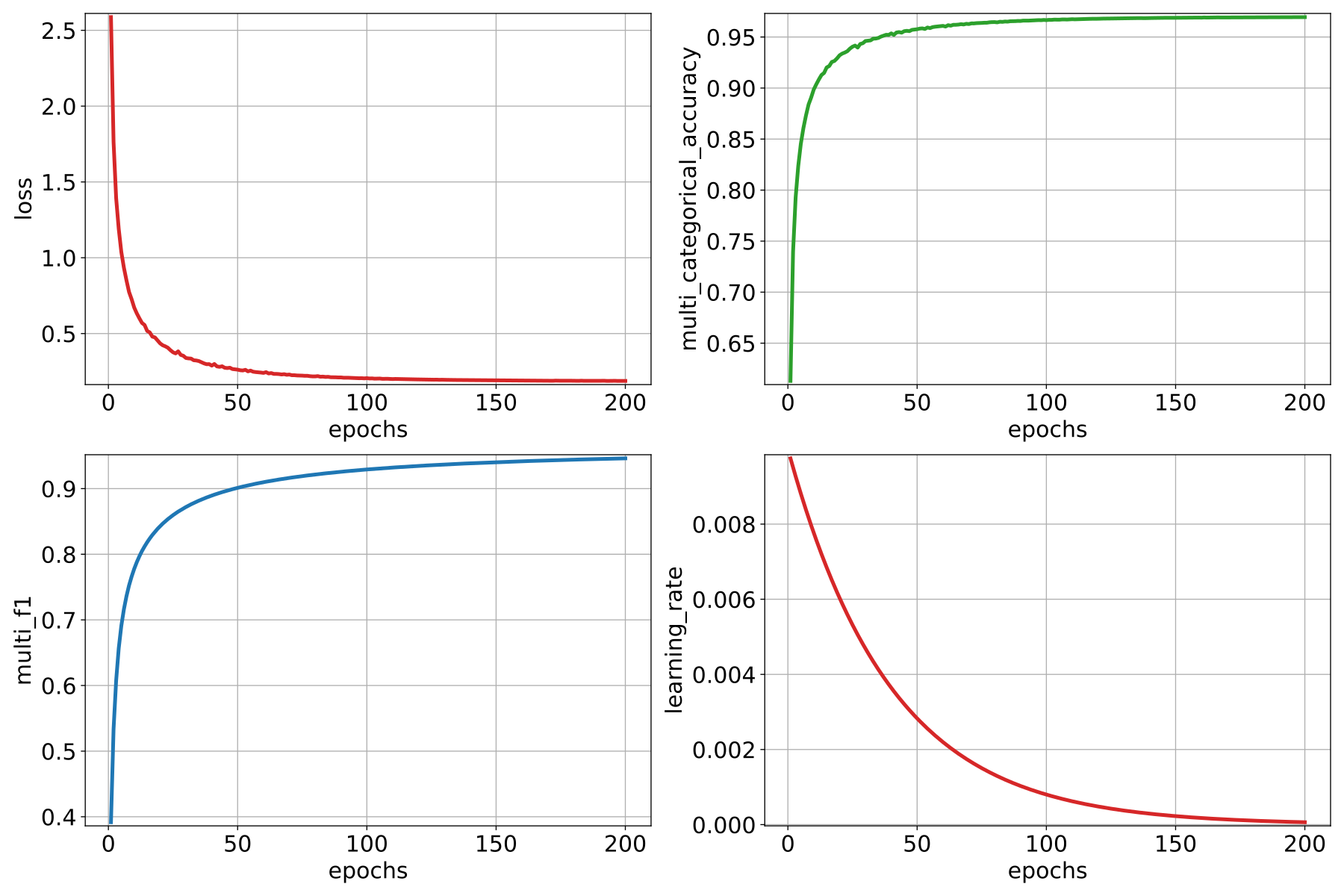
Visualization of the categorical accuracy, the F1-score, the multihead loss, and the learning rate among \(200\) epochs.

Predictive pipeline

The predictive pipeline will use the model on a validation point cloud from the same dataset and epoch. The predictions will be evaluated through ClassificationEvaluator and they will be exported together with their uncertainties through ClassificationUncertaintyEvaluator.

The JSON below corresponds to the described predictive pipeline.

{
  "in_pcloud": [
    "/ext4/hei/Hessigheim_Benchmark/Epoch_March2018/vl3d/mined/Mar18_val_hsv_std.laz"
  ],
  "out_pcloud": [
    "/ext4/hei/Hessigheim_Benchmark/Epoch_March2018/vl3d/out/pointmlp_dumean_neck_multictxhead/T1/preds/*"
  ],
  "sequential_pipeline": [
    {
      "predict": "PredictivePipeline",
      "model_path": "/ext4/hei/Hessigheim_Benchmark/Epoch_March2018/vl3d/out/pointmlp_dumean_neck_multictxhead/T1/model/PointMLP.pipe"
    },
    {
      "eval": "ClassificationEvaluator",
      "class_names": ["LowVeg", "ImpSurf", "Vehicle", "UrbanFurni", "Roof", "Facade", "Shrub", "Tree", "Soil/Gravel", "VertSurf", "Chimney"],
      "metrics": ["OA", "P", "R", "F1", "IoU", "wP", "wR", "wF1", "wIoU", "MCC", "Kappa"],
      "class_metrics": ["P", "R", "F1", "IoU"],
      "confusion_matrix_normalization_strategy": "row",
      "report_path": "*report/global_eval.log",
      "class_report_path": "*report/class_eval.log",
      "confusion_matrix_report_path" : "*report/confusion_matrix.log",
      "confusion_matrix_plot_path" : "*plot/confusion_matrix.svg",
      "class_distribution_report_path": "*report/class_distribution.log",
      "class_distribution_plot_path": "*plot/class_distribution.svg"
    },
    {
        "eval": "ClassificationUncertaintyEvaluator",
        "class_names": ["LowVeg", "ImpSurf", "Vehicle", "UrbanFurni", "Roof", "Facade", "Shrub", "Tree", "Soil/Gravel", "VertSurf", "Chimney"],
        "include_probabilities": true,
        "include_weighted_entropy": false,
        "include_clusters": false,
        "weight_by_predictions": false,
        "num_clusters": 0,
        "clustering_max_iters": 128,
        "clustering_batch_size": 1000000,
        "clustering_entropy_weights": false,
        "clustering_reduce_function": null,
        "gaussian_kernel_points": 256,
        "report_path": "*uncertainty/uncertainty.las",
        "plot_path": "*uncertainty/"
    }
  ]
}

The table below represents the global evaluation metrics. It shows the overall accuracy (OA), precision (P), recall (R), F1-score (F1), intersection over union (IoU), all of them weighted by the number of points, the Matthew’s correlation coefficient (MCC), and the Cohen’s Kappa score (Kappa).

OA	P	R	F1	IoU	wP	wR	wF1	wIoU	MCC	Kappa
84.191	75.574	55.031	58.040	46.434	83.849	84.191	82.553	73.539	80.456	80.280

The figure below shows the reference and predicted labels, the class ambiguity as a point-wise uncertainty measurement, and the binary error mask (gray for correctly classified points, red for misclassified ones).

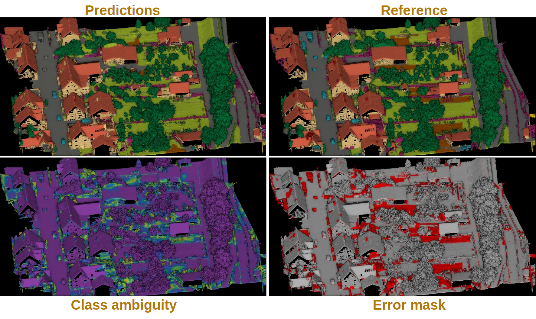
Visualization of the semantic segmentation model applied to previously unseen data. The bottom-right image shows correctly classified points in gray and misclassified points in red. The predictions and reference image use the same color code for the classes. The class ambiguity is represented with purple color for low-uncertainty regions and yellow for high-uncertainty ones.

KPConvX-based model

This example shows how to define two different pipelines, one to train a KPCovnX-based model (see Hierarchical KPConvX documentation) and export it as a PredictivePipeline, the other to use the predictive pipeline to compute a semantic segmentation on a previously unseen point cloud. Readers are referred to the pipelines documentation to read more about how pipelines work and to see more examples.

Training pipeline

The training pipeline will train a ConvAutoencPwiseClassif for the multiclass semantic segmentation of the points. The training point cloud is generated from the March 2018 training point cloud in the Hessigheim dataset by transforming the RGB color components to its HSV representation with HSV from RGB miner.

The pre-processing strategy computes \(25,000\) receptive fields with \(4096\) points at the first depth taken from a spherical neighborhood with a radius of \(5\) meters. It uses an oversampling strategy based on nearest neighbors to puplate receptive fields with not enough points.

The first downsampling (i.e., the one that maps the original input neighborhood to the first receptive field) considers the closest neighbor. Subsequent receptive fields consider the mean of the \(16\) closest neighbors when downsampling. The upsampling layers work with the same number of nearest neighbors.

Note that the neighborhoods are configured in a different way than usual. In general this example is further from the original KPConvX architecture compared to the one in the Hierarchical KPConvX documentation. Another important difference is the lack of KPConvXLayer elements in the decoding stages.

The JSON below corresponds to the described training pipeline.

{
    "in_pcloud": [
        "/ext4/hei/Hessigheim_Benchmark/Epoch_March2018/vl3d/mined/Mar18_train_hsv_std.laz"
    ],
    "out_pcloud": [
        "/ext4/hei/Hessigheim_Benchmark/Epoch_March2018/vl3d/out/kpconvx_dumean_neck/T1/*"
    ],
    "sequential_pipeline": [
        {
            "train": "ConvolutionalAutoencoderPwiseClassifier",
            "training_type": "base",
            "fnames": ["ones", "HSV_Hrad", "HSV_S", "HSV_V"],
            "random_seed": null,
            "model_args": {
                "fnames": ["ones", "HSV_Hrad", "HSV_S", "HSV_V"],
                "num_classes": 11,
                "class_names": ["LowVeg", "ImpSurf", "Vehicle", "UrbanFurni", "Roof", "Facade", "Shrub", "Tree", "Soil/Gravel", "VertSurf", "Chimney"],
                "pre_processing": {
                    "pre_processor": "hierarchical_fpspp",
                    "support_strategy_num_points": 25000,
                    "to_unit_sphere": false,
                    "support_strategy": "fps",
                    "support_strategy_fast": 2,
                    "min_distance": 0.03,
                    "receptive_field_oversampling": {
                        "min_points": 2,
                        "strategy": "nearest",
                        "k": 3,
                        "radius": 0.5
                    },
                    "center_on_pcloud": true,
                    "training_class_distribution": [2250, 2250, 2250, 2250, 2250, 2250, 2250, 2250, 2250, 2250, 2250],
                    "neighborhood": {
                        "type": "sphere",
                        "radius": 5.0,
                        "separation_factor": 0.8
                    },
                    "num_points_per_depth": [4096, 1024, 256, 64, 16],
                    "fast_flag_per_depth": [4, 4, false, false, false],
                    "num_downsampling_neighbors": [1, 16, 16, 16, 16],
                    "num_pwise_neighbors": [16, 16, 16, 16, 16],
                    "num_upsampling_neighbors": [1, 16, 16, 16, 16],
                    "nthreads": -1,
                    "training_receptive_fields_distribution_report_path": null,
                    "training_receptive_fields_distribution_plot_path": null,
                    "training_receptive_fields_dir": null,
                    "receptive_fields_distribution_report_path": null,
                    "receptive_fields_distribution_plot_path": null,
                    "receptive_fields_dir": null,
                    "training_support_points_report_path": null,
                    "support_points_report_path": null
                },
                "feature_extraction": {
                    "type": "KPConvX",
                    "kpconv":{
                        "feature_space_dims": 64,
                        "sigma": 5.0,
                        "kernel_radius": 5.0,
                        "num_kernel_points": 17,
                        "deformable": false,
                        "W_initializer": "he_uniform",
                        "W_regularizer": null,
                        "W_constraint": null,
                        "bn": true,
                        "bn_momentum": 0.90,
                        "activate": true
                    },
                    "operations_per_depth": [1, 1, 1, 1, 1],
                    "blocks": [3, 3, 9, 12, 3],
                    "feature_space_dims": [64, 96, 128, 192, 256],
                    "hidden_feature_space_dims": [256, 384, 512, 768, 1024],
                    "sigma": [5.0, 5.0, 5.0, 5.0, 5.0],
                    "shell_radii": [[0, 2.5, 5.0], [0, 2.5, 5.0], [0, 2.5, 5.0], [0, 2.5, 5.0], [0, 2.5, 5.0]],
                    "shell_points": [[1, 14, 28], [1, 14, 28], [1, 14, 28], [1, 14, 28], [1, 14, 28]],
                    "bn": [true, true, true, true, true],
                    "bn_momentum": [0.90, 0.90, 0.90, 0.90, 0.90],
                    "activate": [true, true, true, true, true],
                    "groups": [8, 8, 8, 8, 8],
                    "deformable": [false, false, false, false, false],
                    "initializer": ["he_uniform", "he_uniform", "he_uniform", "he_uniform", "he_uniform"],
                    "regularizer": [null, null, null, null, null],
                    "constraint": [null, null, null, null, null]
                },
                "features_alignment": null,
                "downsampling_filter": "mean",
                "upsampling_filter": "mean",
                "upsampling_bn": true,
                "upsampling_momentum": 0.90,
                "conv1d": true,
                "conv1d_kernel_initializer": "he_uniform",
                "neck":{
                    "max_depth": 2,
                    "hidden_channels": [64, 64],
                    "kernel_initializer": ["he_uniform", "he_uniform"],
                    "kernel_regularizer": [null, null],
                    "kernel_constraint": [null, null],
                    "bn_momentum": [0.90, 0.90],
                    "activation": ["relu", "relu"]
                },
                "output_kernel_initializer": "he_normal",
                "model_handling": {
                    "summary_report_path": "*/model_summary.log",
                    "training_history_dir": "*/training_eval/history",
                    "class_weight": [1.0, 1.0, 1.0, 1.0, 1.0, 1.0, 1.0, 1.0, 1.0, 1.0, 1.0],
                    "training_epochs": 200,
                    "batch_size": 16,
                    "training_sequencer": {
                        "type": "DLSequencer",
                        "random_shuffle_indices": true,
                        "augmentor": {
                            "transformations": [
                                    {
                                        "type": "Rotation",
                                        "axis": [0, 0, 1],
                                        "angle_distribution": {
                                            "type": "uniform",
                                            "start": -3.141592,
                                            "end": 3.141592
                                        }
                                    },
                                    {
                                        "type": "Scale",
                                        "scale_distribution": {
                                            "type": "uniform",
                                            "start": 0.985,
                                            "end": 1.015
                                        }
                                    },
                                    {
                                        "type": "Jitter",
                                        "noise_distribution": {
                                            "type": "normal",
                                            "mean": 0,
                                            "stdev": 0.0033
                                        }
                                    }
                            ]
                        }
                    },
                    "prediction_reducer": {
                        "reduce_strategy" : {
                            "type": "MeanPredReduceStrategy"
                        },
                        "select_strategy": {
                            "type": "ArgMaxPredSelectStrategy"
                        }
                    },
                    "checkpoint_path": "*/checkpoint.weights.h5",
                    "checkpoint_monitor": "loss",
                    "learning_rate_on_plateau": {
                        "monitor": "loss",
                        "mode": "min",
                        "factor": 0.1,
                        "patience": 2000,
                        "cooldown": 5,
                        "min_delta": 0.01,
                        "min_lr": 1e-6
                    }
                },
                "compilation_args": {
                    "optimizer": {
                        "algorithm": "AdamW",
                        "learning_rate": {
                            "schedule": "exponential_decay",
                            "schedule_args": {
                                "initial_learning_rate": 1e-2,
                                "decay_steps": 2500,
                                "decay_rate": 0.96,
                                "staircase": false
                            }
                        }
                    },
                    "loss": {
                        "function": "class_weighted_categorical_crossentropy"
                    },
                    "metrics": [
                        "categorical_accuracy",
                        "f1"
                    ]
                },
                "architecture_graph_path": "*/model_graph.png",
                "architecture_graph_args": {
                    "show_shapes": true,
                    "show_dtype": true,
                    "show_layer_names": true,
                    "rankdir": "TB",
                    "expand_nested": true,
                    "dpi": 300,
                    "show_layer_activations": true
                }
            },
            "autoval_metrics": null,
            "training_evaluation_metrics": null,
            "training_class_evaluation_metrics": null,
            "training_evaluation_report_path": null,
            "training_class_evaluation_report_path": null,
            "training_confusion_matrix_report_path": null,
            "training_confusion_matrix_plot_path": null,
            "training_class_distribution_report_path": null,
            "training_class_distribution_plot_path": null,
            "training_classified_point_cloud_path": null,
            "training_activations_path": null
        },
        {
            "writer": "PredictivePipelineWriter",
            "out_pipeline": "*/model/KPConvX.pipe",
            "include_writer": false,
            "include_imputer": true,
            "include_feature_transformer": true,
            "include_miner": true,
            "include_class_transformer": false,
            "include_clustering": false,
            "ignore_predictions": false
        }
    ]
}

The figure below represents the evolution among the many training epochs of the categorical accuracy, the F1-score, the loss function, and the learning rate.

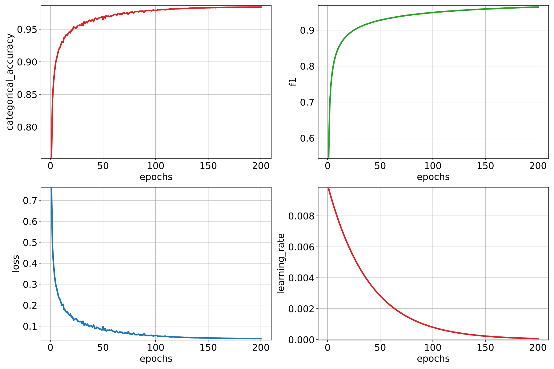
Visualization of the categorical accuracy, the F1-score, the loss, and the learning rate among \(200\) epochs.

Predictive pipeline

The predictive pipeline will use the model on a validation point cloud from the same dataset and epoch. The predictions will be evaluated through ClassificationEvaluator and they will be exported together with their uncertainties through ClassificationUncertaintyEvaluator.

The JSON below corresponds to the described predictive pipeline.

{
  "in_pcloud": [
    "/ext4/hei/Hessigheim_Benchmark/Epoch_March2018/vl3d/mined/Mar18_val_hsv_std.laz"
  ],
  "out_pcloud": [
    "/ext4/hei/Hessigheim_Benchmark/Epoch_March2018/vl3d/out/kpconvx_dumean_neck/T1/preds/*"
  ],
  "sequential_pipeline": [
    {
      "predict": "PredictivePipeline",
      "model_path": "/ext4/hei/Hessigheim_Benchmark/Epoch_March2018/vl3d/out/kpconvx_dumean_neck/T1/model/KPConvX.pipe"
    },
    {
      "eval": "ClassificationEvaluator",
      "class_names": ["LowVeg", "ImpSurf", "Vehicle", "UrbanFurni", "Roof", "Facade", "Shrub", "Tree", "Soil/Gravel", "VertSurf", "Chimney"],
      "metrics": ["OA", "P", "R", "F1", "IoU", "wP", "wR", "wF1", "wIoU", "MCC", "Kappa"],
      "class_metrics": ["P", "R", "F1", "IoU"],
      "confusion_matrix_normalization_strategy": "row",
      "report_path": "*report/global_eval.log",
      "class_report_path": "*report/class_eval.log",
      "confusion_matrix_report_path" : "*report/confusion_matrix.log",
      "confusion_matrix_plot_path" : "*plot/confusion_matrix.svg",
      "class_distribution_report_path": "*report/class_distribution.log",
      "class_distribution_plot_path": "*plot/class_distribution.svg"
    },
    {
        "eval": "ClassificationUncertaintyEvaluator",
        "class_names": ["LowVeg", "ImpSurf", "Vehicle", "UrbanFurni", "Roof", "Facade", "Shrub", "Tree", "Soil/Gravel", "VertSurf", "Chimney"],
        "include_probabilities": true,
        "include_weighted_entropy": false,
        "include_clusters": false,
        "weight_by_predictions": false,
        "num_clusters": 0,
        "clustering_max_iters": 0,
        "clustering_batch_size": 0,
        "clustering_entropy_weights": false,
        "clustering_reduce_function": null,
        "gaussian_kernel_points": 256,
        "report_path": "*uncertainty/uncertainty.las",
        "plot_path": "*uncertainty/"
    }
  ]
}

The table below represents the global evaluation metrics. It shows the overall accuracy (OA), precision (P), recall (R), F1-score (F1), intersection over union (IoU), all of them weighted by the number of points, the Matthew’s correlation coefficient (MCC), and the Cohen’s Kappa score (Kappa).

OA	P	R	F1	IoU	wP	wR	wF1	wIoU	MCC	Kappa
87.368	82.448	69.158	73.272	61.322	86.719	87.368	86.563	78.426	84.346	84.294

The figure below shows the reference and predicted labels, the class ambiguity as a point-wise uncertainty measurement, and the binary error mask (gray for correctly classified points, red for misclassified ones).

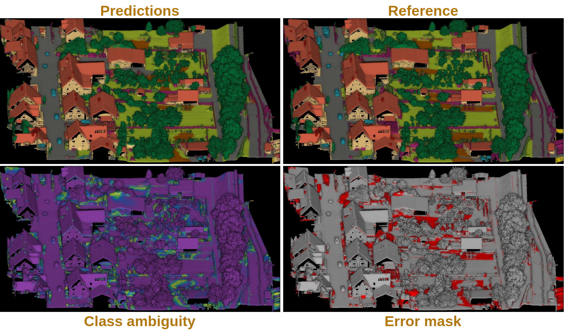
Visualization of the semantic segmentation model applied to previously unseen data. The bottom-right image shows correctly classified points in gray and misclassified points in red. The predictions and reference images use the same color code for the classes. The class ambiguity is represented with purple color for low-uncertainty regions and yellow for high-uncertainty ones.

ContextNet-based model

This example shows how to define two different pipelines, one to train a ContextNet-based model (see Hierarchical ContextNet documentation) and export it as a PredictivePipeline, the other to use the predictive pipeline to compute a semantic segmentation on a previously unseen point cloud. Readers are referred to the pipelines documentation to read more about how pipelines work and to see more examples.

Training pipeline

The training pipeline will train a ConvAutoencPwiseClassif for the multiclass semantic segmentation of the points. The training point cloud is generated from the March 2018 training point cloud in the Hessigheim dataset by transforming the RGB color components to its HSV representation with HSV from RGB miner.

The pre-processing strategy computes \(25,000\) receptive fields with \(4096\) points at the first depth taken from a spherical neighborhood with a radius of \(5\) meters. It uses an oversampling strategy based on nearest neighbors to puplate receptive fields with not enough points.

The first downsampling (i.e., the one that maps the original input neighborhood to the first receptive field) considers the closest neighbor. Subsequent receptive fields consider the mean of the \(16\) closest neighbors when downsampling. The upsampling layers work with the same number of nearest neighbors.

Note that this version of ContextNet uses a multihead contextual head.

The JSON below corresponds to the described training pipeline.

{
    "in_pcloud": [
        "/ext4/hei/Hessigheim_Benchmark/Epoch_March2018/vl3d/mined/Mar18_train_hsv_std.laz"
    ],
    "out_pcloud": [
        "/ext4/hei/Hessigheim_Benchmark/Epoch_March2018/vl3d/out/contextual_dumean_hourglass_neck_multihead/T1/*"
    ],
    "sequential_pipeline": [
        {
            "train": "ConvolutionalAutoencoderPwiseClassifier",
            "training_type": "base",
            "fnames": ["ones", "HSV_Hrad", "HSV_S", "HSV_V"],
            "random_seed": null,
            "model_args": {
                "fnames": ["ones", "HSV_Hrad", "HSV_S", "HSV_V"],
                "num_classes": 11,
                "class_names": ["LowVeg", "ImpSurf", "Vehicle", "UrbanFurni", "Roof", "Facade", "Shrub", "Tree", "Soil/Gravel", "VertSurf", "Chimney"],
                "pre_processing": {
                    "pre_processor": "hierarchical_fpspp",
                    "support_strategy_num_points": 25000,
                    "to_unit_sphere": false,
                    "support_strategy": "fps",
                    "support_strategy_fast": 2,
                    "min_distance": 0.03,
                    "receptive_field_oversampling": {
                        "min_points": 2,
                        "strategy": "nearest",
                        "k": 3,
                        "radius": 0.5
                    },
                    "center_on_pcloud": true,
                    "training_class_distribution": [2250, 2250, 2250, 2250, 2250, 2250, 2250, 2250, 2250, 2250, 2250],
                    "neighborhood": {
                        "type": "sphere",
                        "radius": 5.0,
                        "separation_factor": 0.8
                    },
                    "num_points_per_depth": [4096, 1024, 256, 64, 16],
                    "fast_flag_per_depth": [4, 4, false, false, false],
                    "num_downsampling_neighbors": [1, 16, 16, 16, 16],
                    "num_pwise_neighbors": [16, 16, 16, 16, 16],
                    "num_upsampling_neighbors": [1, 16, 16, 16, 16],
                    "nthreads": -1,
                    "training_receptive_fields_distribution_report_path": null,
                    "training_receptive_fields_distribution_plot_path": null,
                    "training_receptive_fields_dir": null,
                    "receptive_fields_distribution_report_path": null,
                    "receptive_fields_distribution_plot_path": null,
                    "receptive_fields_dir": null,
                    "training_support_points_report_path": null,
                    "support_points_report_path": null
                },
                "feature_extraction": {
                    "type": "Contextual",
                    "operations_per_depth": [2, 1, 1, 1, 1],
                    "feature_space_dims": [64, 64, 96, 128, 192, 256],
                    "hidden_channels": [128, 128, 192, 256, 384, 512],
                    "bn": [true, true, true, true, true, true],
                    "bn_momentum": [0.95, 0.95, 0.95, 0.95, 0.95, 0.95],
                    "bn_along_neighbors": [true, true, true, true, true, true],
                    "activation": ["relu", "relu", "relu", "relu", "relu", "relu"],
                    "distance": ["euclidean", "euclidean", "euclidean", "euclidean", "euclidean", "euclidean"],
                    "ascending_order": [true, true, true, true, true, true],
                    "aggregation": ["mean", "mean", "mean", "mean", "mean", "mean"],
                    "initializer": ["he_uniform", "he_uniform", "he_uniform", "he_uniform", "he_uniform", "he_uniform"],
                    "regularizer": [null, null, null, null, null, null],
                    "constraint": [null, null, null, null, null, null],
                    "activate": true,
                    "hourglass_wrapper": {
                        "internal_dim": [2, 2, 4, 16, 32, 64],
                        "parallel_internal_dim": [8, 8, 16, 32, 64, 128],
                        "activation": ["relu", "relu", "relu", "relu", "relu", "relu"],
                        "activation2": [null, null, null, null, null, null],
                        "regularize": [true, true, true, true, true, true],
                        "W1_initializer": ["he_uniform", "he_uniform", "he_uniform", "he_uniform", "he_uniform", "he_uniform"],
                        "W1_regularizer": [null, null, null, null, null, null],
                        "W1_constraint": [null, null, null, null, null, null],
                        "W2_initializer": ["he_uniform", "he_uniform", "he_uniform", "he_uniform", "he_uniform", "he_uniform"],
                        "W2_regularizer": [null, null, null, null, null, null],
                        "W2_constraint": [null, null, null, null, null, null],
                        "loss_factor": 0.1,
                        "subspace_factor": 0.125,
                        "feature_dim_divisor": 4,
                        "bn": false,
                        "bn_momentum": 0.95,
                        "out_bn": true,
                        "out_bn_momentum": 0.95,
                        "out_activation": "relu"
                    }
                },
                "features_alignment": null,
                "downsampling_filter": "mean",
                "upsampling_filter": "mean",
                "upsampling_bn": true,
                "upsampling_momentum": 0.95,
                "upsampling_hourglass": {
                    "activation": "relu",
                    "activation2": null,
                    "regularize": true,
                    "W1_initializer": "he_uniform",
                    "W1_regularizer": null,
                    "W1_constraint": null,
                    "W2_initializer": "he_uniform",
                    "W2_regularizer": null,
                    "W2_constraint": null,
                    "loss_factor": 0.1,
                    "subspace_factor": 0.125
                },
                "conv1d": false,
                "conv1d_kernel_initializer": "he_uniform",
                "neck":{
                    "max_depth": 2,
                    "hidden_channels": [64, 64],
                    "kernel_initializer": ["he_uniform", "he_uniform"],
                    "kernel_regularizer": [null, null],
                    "kernel_constraint": [null, null],
                    "bn_momentum": [0.95, 0.95],
                    "activation": ["relu", "relu"]
                },
                "contextual_head": {
                    "multihead": true,
                    "max_depth": 2,
                    "hidden_channels": [64, 64],
                    "output_channels": [64, 64],
                    "bn": [true, true],
                    "bn_momentum": [0.95, 0.95],
                    "bn_along_neighbors": [true, true],
                    "activation": ["relu", "relu"],
                    "distance": ["euclidean", "euclidean"],
                    "ascending_order": [true, true],
                    "aggregation": ["mean", "mean"],
                    "initializer": ["he_uniform", "he_uniform"],
                    "regularizer": [null, null],
                    "constraint": [null, null]
                },
                "output_kernel_initializer": "he_normal",
                "model_handling": {
                    "summary_report_path": "*/model_summary.log",
                    "training_history_dir": "*/training_eval/history",
                    "class_weight": [1.0, 1.0, 1.0, 1.0, 1.0, 1.0, 1.0, 1.0, 1.0, 1.0, 1.0],
                    "training_epochs": 200,
                    "batch_size": 16,
                    "training_sequencer": {
                        "type": "DLSequencer",
                        "random_shuffle_indices": true,
                        "augmentor": {
                            "transformations": [
                                    {
                                        "type": "Rotation",
                                        "axis": [0, 0, 1],
                                        "angle_distribution": {
                                            "type": "uniform",
                                            "start": -3.141592,
                                            "end": 3.141592
                                        }
                                    },
                                    {
                                        "type": "Scale",
                                        "scale_distribution": {
                                            "type": "uniform",
                                            "start": 0.985,
                                            "end": 1.015
                                        }
                                    },
                                    {
                                        "type": "Jitter",
                                        "noise_distribution": {
                                            "type": "normal",
                                            "mean": 0,
                                            "stdev": 0.0033
                                        }
                                    }
                            ]
                        }
                    },
                    "prediction_reducer": {
                        "reduce_strategy" : {
                            "type": "MeanPredReduceStrategy"
                        },
                        "select_strategy": {
                            "type": "ArgMaxPredSelectStrategy"
                        }
                    },
                    "checkpoint_path": "*/checkpoint.weights.h5",
                    "checkpoint_monitor": "loss",
                    "learning_rate_on_plateau": {
                        "monitor": "loss",
                        "mode": "min",
                        "factor": 0.1,
                        "patience": 2000,
                        "cooldown": 5,
                        "min_delta": 0.01,
                        "min_lr": 1e-6
                    }
                },
                "compilation_args": {
                    "optimizer": {
                        "algorithm": "AdamW",
                        "learning_rate": {
                            "schedule": "exponential_decay",
                            "schedule_args": {
                                "initial_learning_rate": 1e-2,
                                "decay_steps": 2500,
                                "decay_rate": 0.96,
                                "staircase": false
                            }
                        }
                    },
                    "loss": {
                        "function": "class_weighted_categorical_crossentropy"
                    },
                    "metrics": [
                        "categorical_accuracy",
                        "f1"
                    ]
                },
                "architecture_graph_path": "*/model_graph.png",
                "architecture_graph_args": {
                    "show_shapes": true,
                    "show_dtype": false,
                    "show_layer_names": true,
                    "rankdir": "LR",
                    "expand_nested": false,
                    "dpi": 300,
                    "show_layer_activations": false
                }
            },
            "autoval_metrics": null,
            "training_evaluation_metrics": null,
            "training_class_evaluation_metrics": null,
            "training_evaluation_report_path": null,
            "training_class_evaluation_report_path": null,
            "training_confusion_matrix_report_path": null,
            "training_confusion_matrix_plot_path": null,
            "training_class_distribution_report_path": null,
            "training_class_distribution_plot_path": null,
            "training_classified_point_cloud_path": null,
            "training_activations_path": null
        },
        {
            "writer": "PredictivePipelineWriter",
            "out_pipeline": "*/model/ContextNet.pipe",
            "include_writer": false,
            "include_imputer": true,
            "include_feature_transformer": true,
            "include_miner": true,
            "include_class_transformer": false,
            "include_clustering": false,
            "ignore_predictions": false
        }
    ]
}

The figure below represents the evolution among the many training epochs of the categorical accuracy, the F1-score, the loss function, and the learning rate.

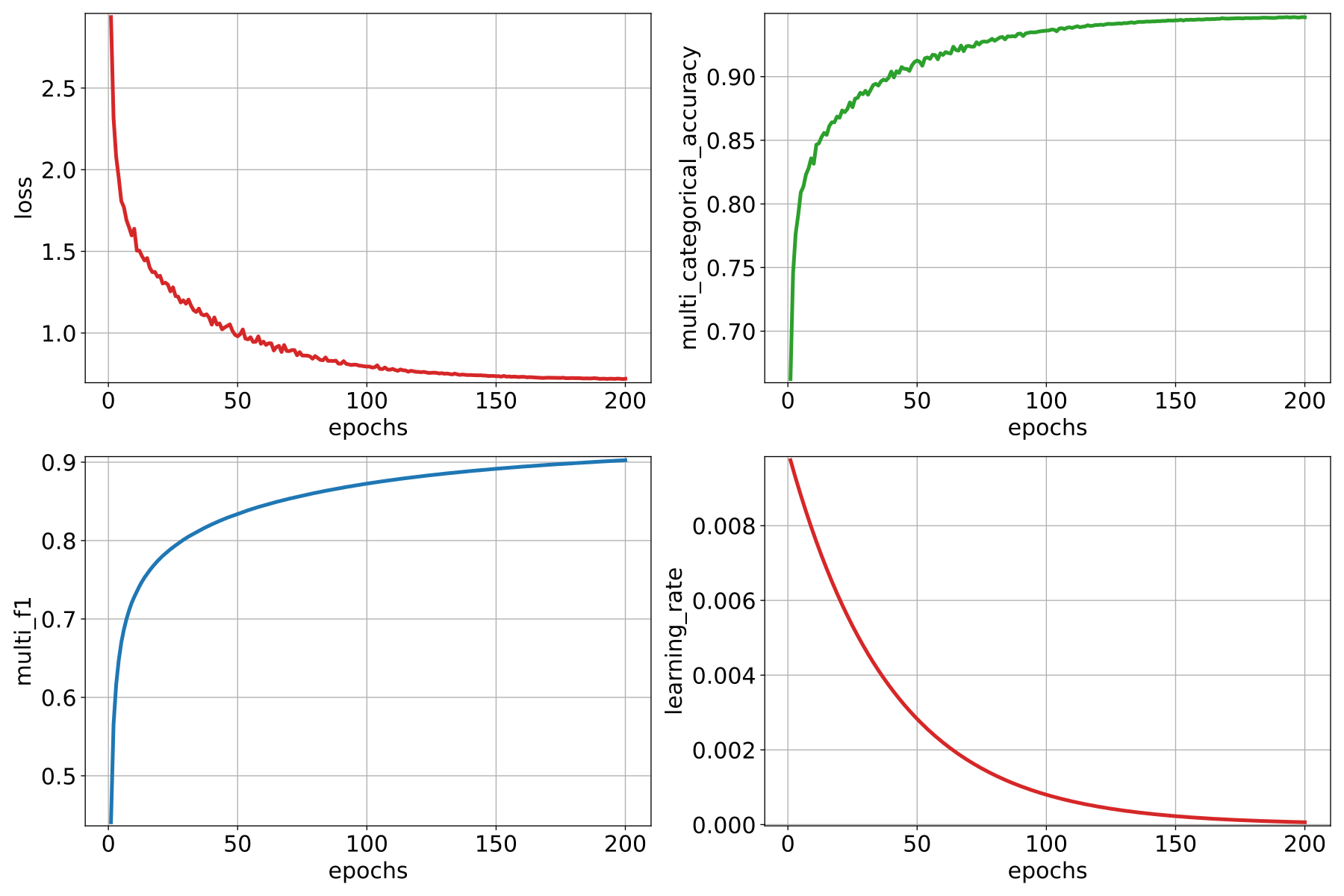
Visualization of the categorical accuracy, the F1-score, the multi-head loss, and the learning rate among \(200\) epochs.

Predictive pipeline

The predictive pipeline will use the model on a validation point cloud from the same dataset and epoch. The predictions will be evaluated through ClassificationEvaluator and they will be exported together with their uncertainties through ClassificationUncertaintyEvaluator.

The JSON below corresponds to the described predictive pipeline.

{
  "in_pcloud": [
    "/ext4/hei/Hessigheim_Benchmark/Epoch_March2018/vl3d/mined/Mar18_val_hsv_std.laz"
  ],
  "out_pcloud": [
    "/ext4/hei/Hessigheim_Benchmark/Epoch_March2018/vl3d/out/contextual_dumean_hourglass_neck_multihead/T1/preds/*"
  ],
  "sequential_pipeline": [
    {
      "predict": "PredictivePipeline",
      "model_path": "/ext4/hei/Hessigheim_Benchmark/Epoch_March2018/vl3d/out/contextual_dumean_hourglass_neck_multihead/T1/model/ContextNet.pipe"
    },
    {
      "eval": "ClassificationEvaluator",
      "class_names": ["LowVeg", "ImpSurf", "Vehicle", "UrbanFurni", "Roof", "Facade", "Shrub", "Tree", "Soil/Gravel", "VertSurf", "Chimney"],
      "metrics": ["OA", "P", "R", "F1", "IoU", "wP", "wR", "wF1", "wIoU", "MCC", "Kappa"],
      "class_metrics": ["P", "R", "F1", "IoU"],
      "confusion_matrix_normalization_strategy": "row",
      "report_path": "*report/global_eval.log",
      "class_report_path": "*report/class_eval.log",
      "confusion_matrix_normalization_strategy": "row",
      "confusion_matrix_report_path" : "*report/confusion_matrix.log",
      "confusion_matrix_plot_path" : "*plot/confusion_matrix.svg",
      "class_distribution_report_path": "*report/class_distribution.log",
      "class_distribution_plot_path": "*plot/class_distribution.svg"
    },
    {
        "eval": "ClassificationUncertaintyEvaluator",
        "class_names": ["LowVeg", "ImpSurf", "Vehicle", "UrbanFurni", "Roof", "Facade", "Shrub", "Tree", "Soil/Gravel", "VertSurf", "Chimney"],
        "include_probabilities": true,
        "include_weighted_entropy": false,
        "include_clusters": false,
        "weight_by_predictions": false,
        "num_clusters": 0,
        "clustering_max_iters": 0,
        "clustering_batch_size": 0,
        "clustering_entropy_weights": false,
        "clustering_reduce_function": null,
        "gaussian_kernel_points": 256,
        "report_path": "*uncertainty/uncertainty.las",
        "plot_path": "*uncertainty/"
    }
  ]
}

The table below represents the global evaluation metrics. It shows the overall accuracy (OA), precision (P), recall (R), F1-score (F1), the intersection over union (IoU), all of them weighted by the number of points, the Matthew’s correlation coefficient (MCC), and the Cohen’s Kappa score (Kappa).

OA	P	R	F1	IoU	wP	wR	wF1	wIoU	MCC	Kappa
87.117	80.441	71.620	74.739	62.081	86.841	87.117	86.689	78.125	84.066	84.019

The figure below shows the reference and predicted labels, the class ambiguity as a point-wise uncertainty measurement, and the binary error mask (gray for correctly classified points, red for misclassified ones).

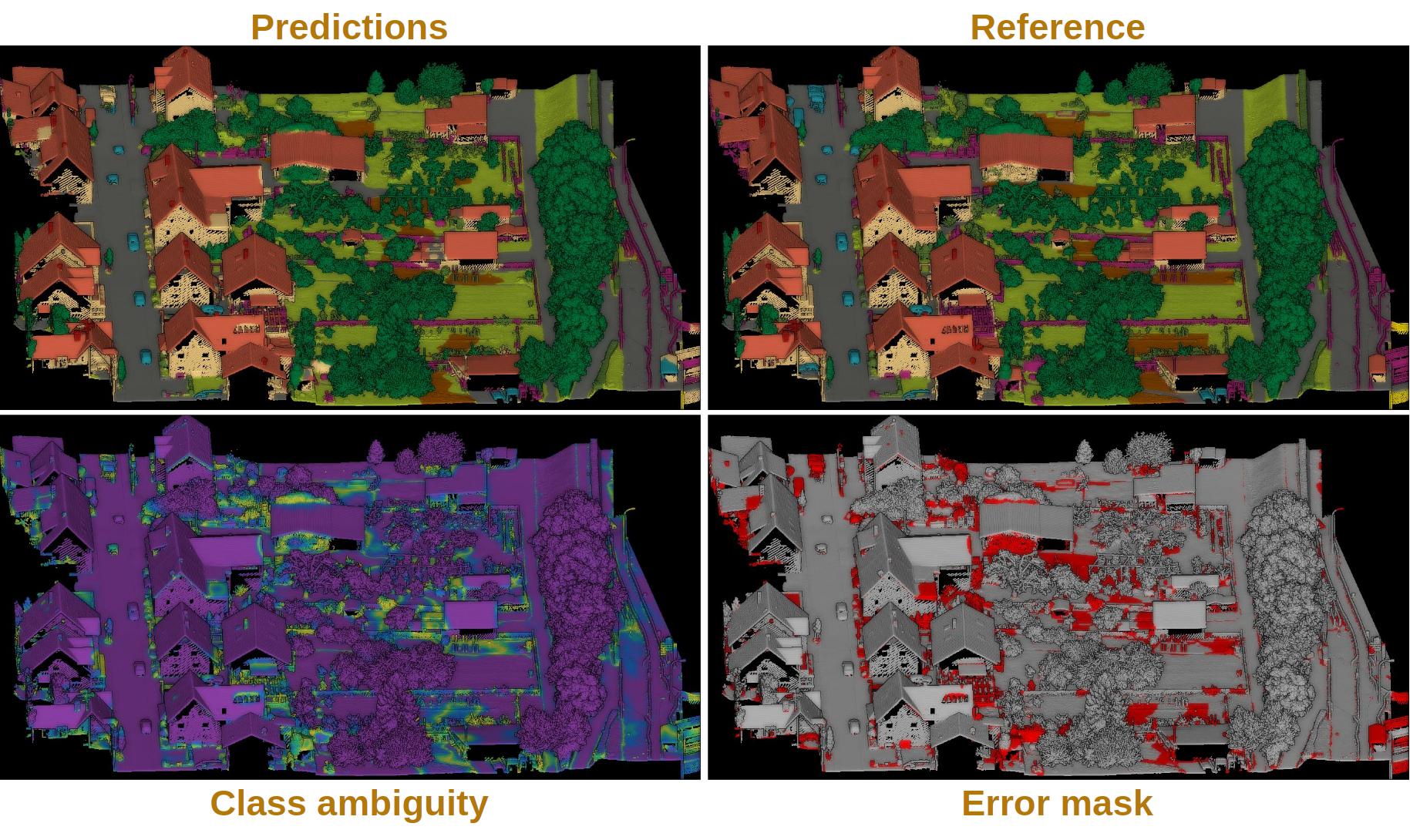
Visualization of the semantic segmentation model applied to previously unseen data. The bottom-right image shows correctly classified points in gray and misclassified points in red. The predictions and reference images use the same color code for the classes. The class ambiguity is represented with purple color for low-uncertainty regions and yellow for high-uncertainty ones.