Evaluators

Evaluators are components that can be used to evaluate the data, the model, or the predictions. The evaluations are typically represented through text reports, point clouds, and plots. An Evaluator component is typically used inside pipelines to assess the performance of a machine learning model or to understand the insights of a neural network. Readers should be familiar with pipelines to understand how to include evaluators in their workflows.

Classification evaluator

The ClassificationEvaluator assumes there is a labeled point cloud and that some predictions have been computed for that point cloud. It will consider the predictions and reference labels at the current pipeline’s state and will evaluate them in different ways. A ClassificationEvaluator can be defined inside a pipeline using the JSON below:

{
    "eval": "ClassificationEvaluator",
    "class_names": ["Ground", "Vegetation", "Building", "Urban furniture", "Vehicle"],
    "metrics": ["OA", "mAcc", "P", "R", "F1", "IoU", "wP", "wR", "wF1", "wIoU", "MCC", "Kappa"],
    "class_metrics": ["Acc", "P", "R", "F1", "IoU"],
    "report_path": "*report/global_eval.log",
    "class_report_path": "*report/class_eval.log",
    "confusion_matrix_report_path" : "confusion_matrix.log",
    "confusion_matrix_plot_path" : "confusion_matrix.svg",
    "confusion_matrix_normalization_strategy": null,
    "class_distribution_report_path": "class_distribution.log",
    "class_distribution_plot_path": "class_distribution.svg",
    "nthreads": 1
}

The JSON above defines a ClassificationEvaluator that will consider many metrics, from the overall accuracy to the Cohen’s kappa score, to evaluate the predicted point clouds. Some metrics will also be considered to compute class-wise scores. On top of that, the confusion matrix and the distribution of the points among the classes will be analyzed. All the evaluations can be exported as a report, typically a text file containing the data or a plot for quick visualization.

Arguments

– class_names

A list with the names for the classes. These names will be used to represent the classes in the plots and the reports.

– metrics

The metrics to evaluate the classification. Supported metrics are:

• "OA" Overall accuracy.

• "mAcc" Mean accuracy.

• "P" Precision.

• "R" Recall.

• "F1" F1 score (harmonic mean of precision and recall).

• "IoU" Intersection over union (also known as Jaccard index).

• "wP" Weighted precision (weights by the number of true instances for each class).

• "wR" Weighted recall (weights by the number of true instances for each class).

• "wF1" Weighted F1 score (weights by the number of true instances for each class).

• "wIoU" Weighted intersection over union (weights by the number of true instances for each class).

• "MCC" Matthews correlation coefficient.

• "Kappa" Cohen’s kappa score.

– class_metrics

The metrics to evaluate the classification in a class-wise way. Supported class metrics are:

• "Acc" Accuracy.

• "P" Precision.

• "R" Recall.

• "F1" F1 score (harmonic mean of precision and recall).

• "IoU" Intersection over union (also known as Jaccard index).

– ignore_classes

Optional list of classes to be ignored when computing the evaluation metrics. Any point whose label matches a class in this list will be excluded. The classes must be given as a list of strings that matches those from class_names, i.e., ignore_classes \(\subseteq\) class_names.

– ignore_predictions

Whether to also ignore the classes in the predictions (true) or not (false, default). Note that it is strongly recommended to avoid ignoring the predictions, as it can lead to wrong interpretations of the model performance. Yet, it can be useful in some circumstances.

– report_path

Path to write the evaluation of the classification to a text file.

– class_report_path

Path to write the class-wise evaluation of the classification to a text file.

– confusion_matrix_report_path

Path to write the confusion matrix to a text file.

– confusion_matrix_plot_path

Path to write the plot representing a confusion matrix to a file.

– confusion_matrix_normalization_strategy

The strategy to normalize the confusion matrix (when plotting it), if any. It can be either "row" to apply a row-wise normalization (i.e., by references, recall), "col" to apply a column-wise normalization (i.e., by predictions, precision), or "full" to normalize considering the total number of samples. When not given (i.e., null), no normalization will be applied.

– class_distribution_report_path

Path to write the class distribution report to a text file.

– class_distribution_plot_path

Path to write the plot representing the class distribution to a file.

– nthreads

The number of threads to use for the parallel computation of evaluation metrics. At most one thread per requested metric can be used. If set to -1 then as many threads as available cores will be used.

Output

The output is illustrated considering the March 2018 point clouds from the Hessigheim dataset to compute the classification’s evaluation.

The table below represents the confusion matrix exported as a CSV report. The rows represent the true labels, while the columns represent the predictions.

Ground	Vegetation	Building	Urban furniture	Vehicle
7117968	48936	246357	121840	9140
52931	1992443	215502	295401	3853
111624	42669	3499547	67170	215
72761	21997	199058	158505	3068
42451	8250	64580	29340	38642

The image below represents the confusion matrix as a figure. The information in the image is the same than the one in the table but in a different format.

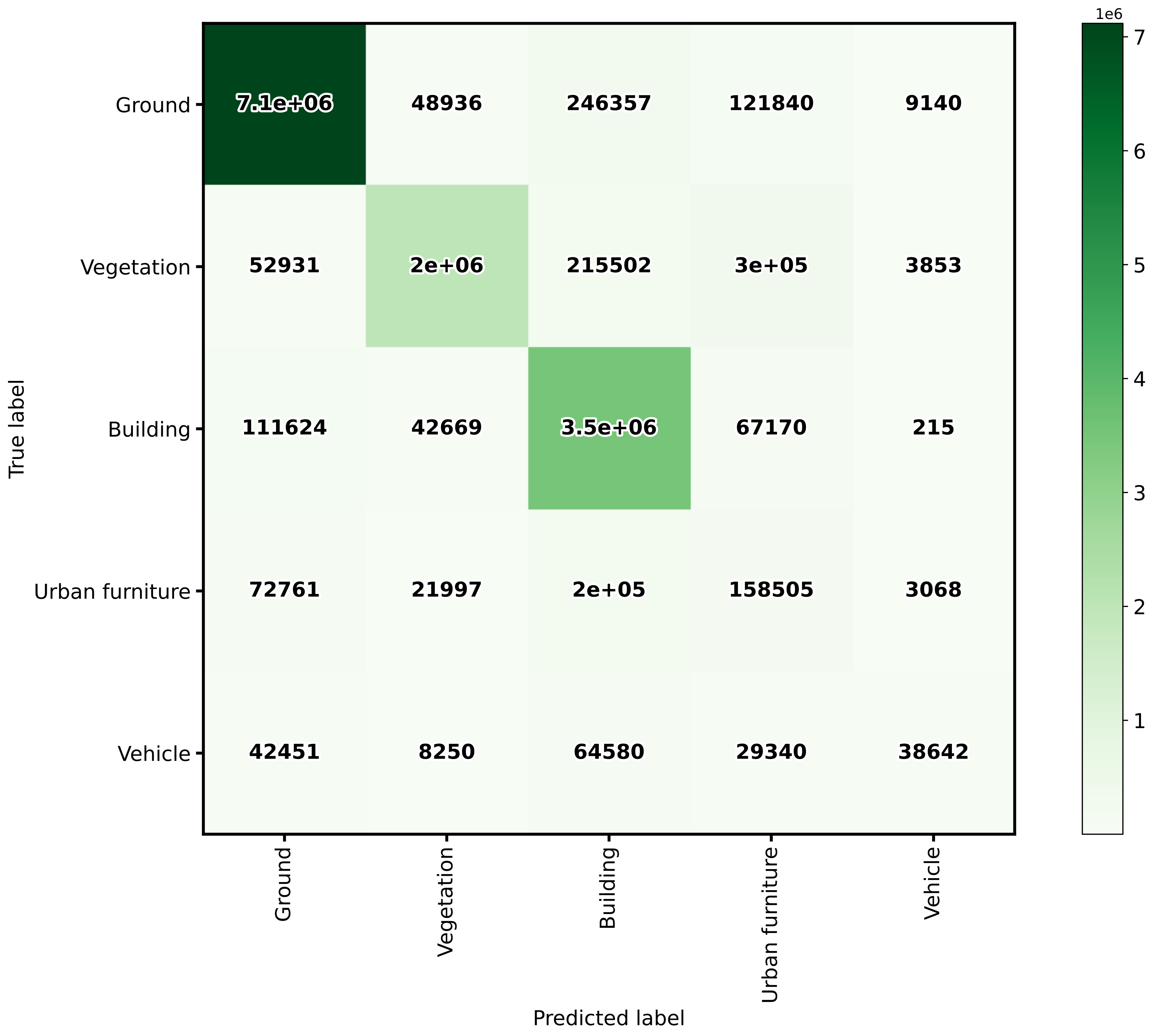
The confusion matrix exported by the classification evaluator.

Advanced classification evaluator

The AdvancedClassificationEvaluator uses the ClassificationEvaluator many times (see documentation), one per node in the analysis domain. It can be defined inside a pipeline using the JSON below:

{
    "eval": "AdvancedClassificationEvaluator",
    "class_names": ["vegetation", "other"],
    "metrics": ["OA", "P", "R", "F1", "IoU", "wP", "wR", "wF1", "wIoU", "MCC", "Kappa"],
    "class_metrics": ["P", "R", "F1", "IoU"],
    "report_path": "*report/global_eval.log",
    "plot_path": "*report/global_plot.svg",
    "class_report_path": "*report/class_eval.log",
    "class_plot_path": "*report/class_eval.svg",
    "confusion_matrix_report_path" : "*report/confusion_matrix.log",
    "confusion_matrix_plot_path" : "*report/confusion_matrix.svg",
    "confusion_matrix_normalization_strategy": "row",
    "class_distribution_report_path": "*report/class_distribution.log",
    "class_distribution_plot_path": "*report/class_distribution.svg",
    "nthreads": 1,
    "domain_name": "PWE cut",
    "filters": [
        {
            "name": "pwe0_1",
            "x": 0.1,
            "conditions": [
                {
                    "value_name": "classification",
                    "condition_type": "equals",
                    "value_target": 2,
                    "action": "discard"
                },
                {
                    "value_name": "PointWiseEntropy",
                    "condition_type": "less_than_or_equal_to",
                    "value_target": 0.1,
                    "action": "preserve"
                }
            ]
        },
        {
            "name": "pwe0_3",
            "x": 0.3,
            "conditions": [
                {
                    "value_name": "classification",
                    "condition_type": "equals",
                    "value_target": 2,
                    "action": "discard"
                },
                {
                    "value_name": "PointWiseEntropy",
                    "condition_type": "less_than_or_equal_to",
                    "value_target": 0.3,
                    "action": "preserve"
                }
            ]
        },
        {
            "name": "pwe0_6",
            "x": 0.6,
            "conditions": [
                {
                    "value_name": "classification",
                    "condition_type": "equals",
                    "value_target": 2,
                    "action": "discard"
                },
                {
                    "value_name": "PointWiseEntropy",
                    "condition_type": "less_than_or_equal_to",
                    "value_target": 0.6,
                    "action": "preserve"
                }
            ]
        },
        {
            "name": "pwe0_9",
            "x": 0.9,
            "conditions": [
                {
                    "value_name": "classification",
                    "condition_type": "equals",
                    "value_target": 2,
                    "action": "discard"
                },
                {
                    "value_name": "PointWiseEntropy",
                    "condition_type": "less_than_or_equal_to",
                    "value_target": 0.9,
                    "action": "preserve"
                }
            ]
        },
        {
            "name": "pwe1",
            "x": 1.0,
            "conditions": [
                {
                    "value_name": "classification",
                    "condition_type": "equals",
                    "value_target": 2,
                    "action": "discard"
                },
                {
                    "value_name": "PointWiseEntropy",
                    "condition_type": "less_than_or_equal_to",
                    "value_target": 1.0,
                    "action": "preserve"
                }
            ]
        }
    ]
}

The JSON above defines a AdvancedClassificationEvaluator that will consider many metrics, for a global evaluation and a class-wise evaluation as well. It will also consider the confusion matrices and the class distributions for each of the four requested nodes in the domain of the "PointWiseEntropy". The confusion matrices will be normalized by references (row-wise). All the evaluations will be exported as a text report but also plots will be generated.

Arguments

– class_names

See classification evaluator documentation .

– metrics

See classification evaluator documentation .

– class_metrics

See classification evaluator documentation .

– ignore_classes

See classification evaluator documentation .

– report_path

See classification evaluator documentation .

– class_report_path

See classification evaluator documentation .

– confusion_matrix_report_path

See classification evaluator documentation .

– confusion_matrix_plot_path

See classification evaluator documentation .

– confusion_matrix_normalization_strategy

See classification evaluator documentation .

– class_distribution_report_path

See classification evaluator documentation .

– class_distribution_plot_path

See classification evaluator documentation .

– nthreads

See classification evaluator documentation .

– domain_name

The name that must be given to the domain (it will be used in the headers of CSV-like output but also in the titles and labels of the generated figures).

– filters

A list with the filters that must be applied, each filter must have a format like shown below:

{
    "name": "filter_name",
    "x": 0.5,
    "conditions": [
        {
            "value_name": "feature_name",
            "condition_type": "less_than_or_equal_to",
            "value_target": 0.5,
            "action": "preserve"
        }
    ]
}

– name

A name for the filter so it can be identified internally when reporting errors.

– x

The value in the domain that corresponds to this node.

– conditions

A list with many conditions specified as dictionaries.

– value_name

The name of the feature (must exist in the point cloud) that must be considered by the filter. It can also be the standard "classification" attribute.

– condition_type

The type of relational that governs the condition. It is one of those that can be specified as the condition types of an advanced input.

– value_target

See value target of an advanced input.

– action

Whether to "preserve" the points that satisfy the condition or to "discard" them.

Output

The output is illustrated using the PNOA-II dataset (in the region of Galicia, northwest Spain). It corresponds to an advanced evaluation like in the example shown above considering the PointWiseEntropy but analyzing linearly spaced nodes from \(0.1\) to \(1.0\) with a step of \(0.1\).

The table below represents the global evaluation metrics exported as a CSV report. The rows represent the metrics for the different point-wise entropy cuts. For each analysis the cut value, the number of points and the many evaluation and correlation metrics are included in the output.

PWE	Points	OA	P	R	F1	IoU	MCC	Kappa
0.1	4495750	97.51	97.00	97.94	97.41	94.95	94.94	94.82
0.2	4951059	96.72	96.44	97.12	96.68	93.58	93.55	93.37
0.3	5133707	96.33	96.12	96.70	96.30	92.86	92.83	92.60
0.4	5231916	96.06	95.90	96.44	96.04	92.38	92.34	92.09
0.5	5308112	95.83	95.69	96.21	95.80	91.95	91.89	91.62
0.6	5400506	95.57	95.45	95.95	95.54	91.47	91.40	91.10
0.7	5561925	95.08	95.02	95.48	95.07	90.60	90.50	90.15
0.8	5729277	94.48	94.47	94.89	94.47	89.52	89.36	88.96
0.9	5890483	93.77	93.81	94.20	93.76	88.25	88.01	87.55
1.0	6251003	91.76	91.84	92.26	91.75	84.75	84.10	83.55

The image below represents the class-wise evaluation on different nodes of the point-wise entropy domain. It can be seen that, no matter the metric and the class, the point-wise entropy is a good uncertainty measurement because the greater it is, the lower the evaluation metric.

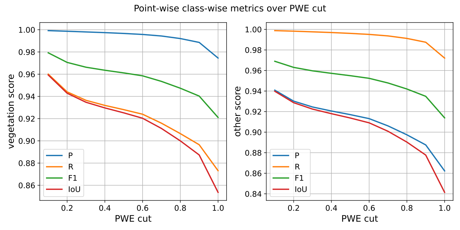
The class-wise evaluation as a function of the point-wise entropy exported by the advanced classification evaluator.

Classification uncertainty evaluator

The ClassificationUncertaintyEvaluator can be used to get insights on what points are more problematic for a given model when solving a particular point-wise classification task. The evaluation will be more detailed when there is more data available (e.g., reference labels) but it can also be computed solely from the predicted probabilities. A ClassificationUncertaintyEvaluator can be defined inside a pipeline using the JSON below:

{
    "eval": "ClassificationUncertaintyEvaluator",
    "class_names": ["Ground", "Vegetation", "Building", "Urban furniture", "Vehicle"],
    "include_probabilities": true,
    "include_weighted_entropy": true,
    "include_clusters": true,
    "weight_by_predictions": false,
    "num_clusters": 10,
    "clustering_max_iters": 128,
    "clustering_batch_size": 1000000,
    "clustering_entropy_weights": true,
    "clustering_reduce_function": "mean",
    "gaussian_kernel_points": 256,
    "report_path": "uncertainty/uncertainty.las",
    "plot_path": "uncertainty/"
}

The JSON above defines a ClassificationUncertaintyEvaluator that will export a point cloud and many plots to the uncertainty directory.

Arguments

– class_names

A list with the names for the classes. These names will be used to represent the classes in the plots and the reports.

– ignore_classes

Optional list of classes to be ignored when computing the uncertainty metrics. Any point whose label matches a class in this list will be excluded. The classes must be given as a list of strings that matches those from class_names, i.e., ignore_classes \(\subseteq\) class_names.

– probability_eps

A value representing the zero. It can be useful to avoid NaNs when computing the logarithms of the likelihoods, i.e., \(\log_2(0)\). If it is exactly zero, then logarithms of zero might arise. Otherwise, the zeroes will be replaced by this value or the minimum greater than zero likelihood, whatever is smaller.

– include_probabilities

Whether to include the probabilities in the output point cloud (True) or not (False).

– include_weighted_entropy

Whether to include the weighted entropy in the evaluation (True) or not (False). The weighted entropy considers either the distribution of reference or predicted labels to compensate for unbalanced class distributions.

– include_clusters

Whether to include the cluster-wise entropy in the evaluation (True) or not (False). Note that the cluster-wise entropy might take too long to compute depending on how it is configured.

– weight_by_predictions

Whether to compute the weighted entropy considering the predictions instead of the reference labels (True) or not (False, by default).

– num_clusters

How many clusters must be computed for the cluster-wise entropy.

– clustering_max_iters

How many iterations are allowed at most when computing the clustering algorithm (KMeans).

– clustering_batch_size

How many points per batch must be considered when computing the batch KMeans.

– clustering_entropy_weights

Whether to use point-wise entropy as the sample weights for the KMeans clustering (True) or not (False).

– clustering_reduce_function

What function must be used to reduce all the entropies in a given cluster to a single one that will be assigned to all points in the cluster. Supported reduce functions are:

• "mean" Select the mean entropy value.

• "median" Select the median of the entropy distribution.

• "Q1" Select the first quartile of the entropy distribution.

• "Q3" Select the third quartile of the entropy distribution.

• "min" Select the min entropy value.

• "max" Select the max entropy value.

– gaussian_kernel_points

How many points will be considered to evaluate each gaussian kernel density estimation.

– report_path

Path to write the point cloud with the computed uncertainty metrics.

– plot_path

Path to the directory where the many plots representing the computed uncertainty metrics will be written.

Output

The output is illustrated considering the March 2018 point clouds from the Hessigheim dataset to compute the classification’s uncertainty evaluation.

Below, an example of one of the figures that can be generated with the ClassificationUncertaintyEvaluator. It clearly illustrates that the point-wise classification of vehicles is problematic.

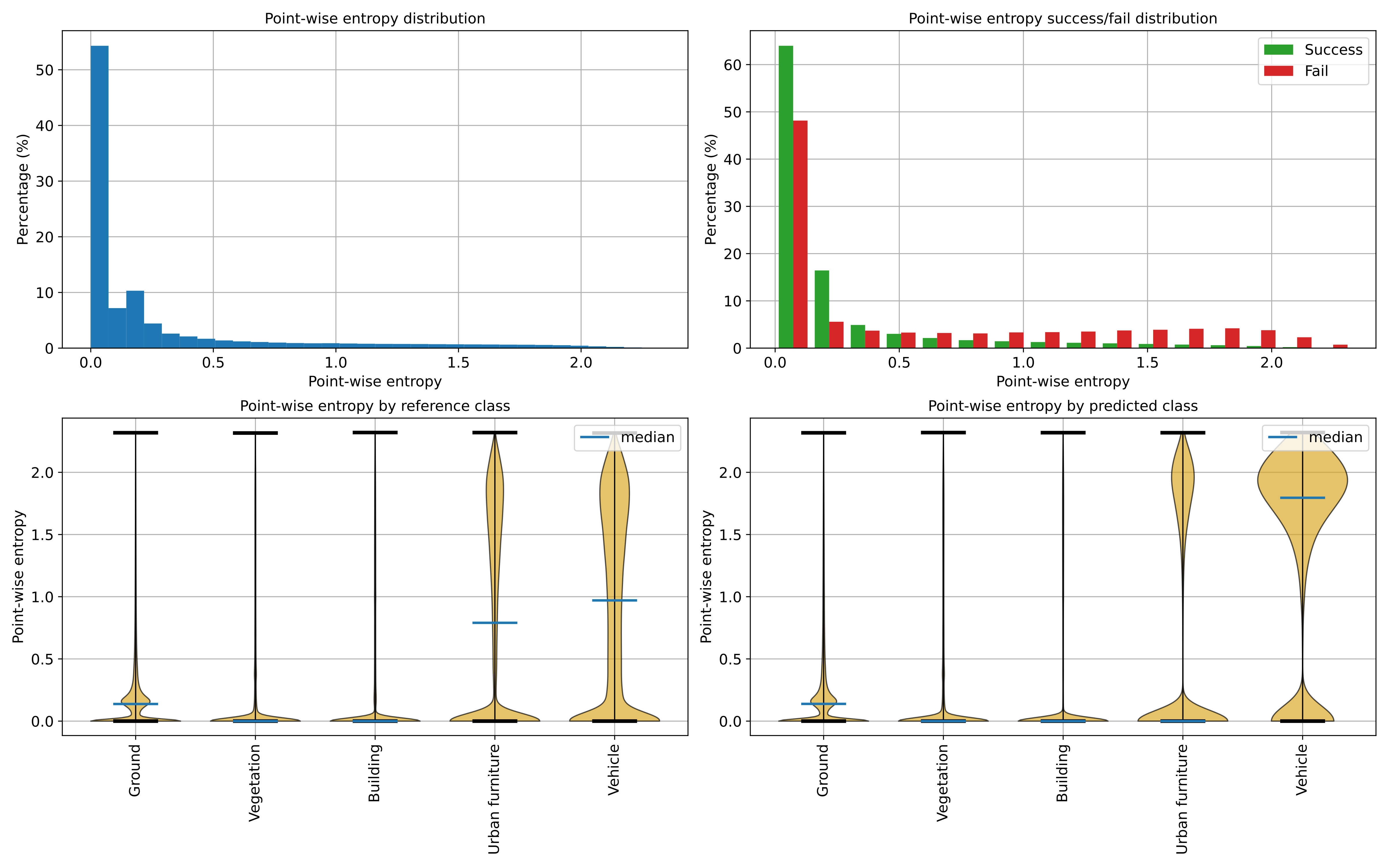
Visualization of the point-wise entropy outside the point cloud.

Below, an example of the point cloud representing the uncertainty metrics. In the general case, it can be seen that a high class ambiguity is associated with misclassified points. Thus, even in the absence of labeled point clouds, the uncertainty metrics can be used to understand the problems of a model when classifying previously unseen data.

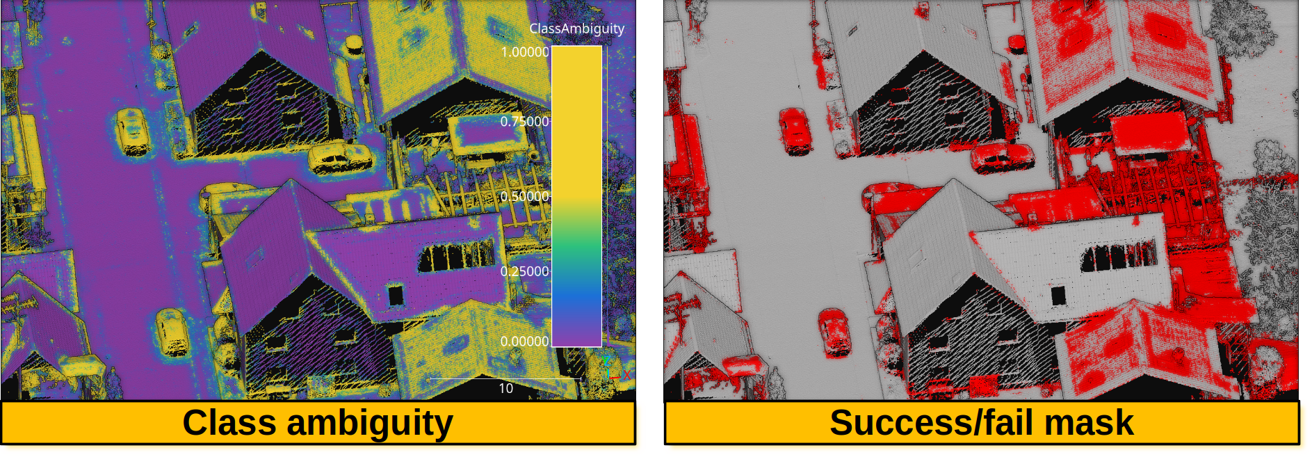
Visualization of a point cloud representing the class ambiguity and the success/fail point-wise mask on previously unseen data, respectively. Red means failed classification and gray means successfully classified.

TORF RF vs NN evaluator

The TORFRFvsNNEvaluator compares the Random Forest (RF) and Neural Network (NN) stages of a trained TransfOctoRFClassificationModel. It independently runs RF and NN inference on the octree centroids, collecting both probability matrices so they can be analyzed side by side. The evaluator produces a multi-panel comparison plot and CSV reports.

The evaluator can be used in two ways:

1. Internally during training by setting rfvsnn_plot_path and/or rfvsnn_report_path inside the TORF training specification (see TransfOctoRF documentation).

2. As a pipeline component after a TORF-based predictive pipeline, which is useful to evaluate predictions on new point clouds with available reference labels.

A TORFRFvsNNEvaluator can be defined inside a pipeline using the JSON below:

{
    "eval": "TORFRFvsNNEvaluator",
    "class_names": ["Ground", "Vegetation", "Building", "Trick"],
    "ignore_classes": ["Trick"],
    "plot_path": "*report/rfvsnn.svg",
    "report_path": "*report/rfvsnn/",
    "pcloud_path": "*report/rfvsnn.las",
    "include_prediction": true,
    "include_class_ambiguity": true,
    "include_probabilities": true
}

The JSON above defines a TORFRFvsNNEvaluator that will generate a comparison plot, CSV reports, and an output point cloud. The evaluator accesses the TORF model from the pipeline state, rebuilds the octree to obtain centroid-level features and labels consistent with training, runs both RF and NN stages on those centroids, and compares their outputs. When a point cloud path is given, centroid-level values are propagated back to the original points via closest-centroid assignment so the output has the same number of points as the input.

Arguments

– class_names

A list with the names for the classes. These names will be used to label the classes in the plots, CSV reports, and point cloud feature names. If not given, the class names from the TORF model will be used.

– ignore_classes

Optional list of class names to exclude from the evaluation. Any centroid whose octree majority-vote label matches an ignored class will be removed before running the RF and NN stages. When a point cloud is exported, original points whose labels match an ignored class are also excluded. The class names must be a subset of class_names, i.e., ignore_classes \(\subseteq\) class_names. When null or not given, all classes are included and the evaluator behaves as if no filtering was requested.

– plot_path

Path to write the multi-panel comparison figure. The figure contains four panels:

• Per-class F1 comparison grouped bar chart showing RF and NN F1 scores side by side for each class.

• Class ambiguity distributions overlapping histograms of RF and NN class ambiguity values.

• Prediction agreement pie chart showing the fraction of centroids where RF and NN agree vs disagree (and who is correct).

• Ambiguity scatter scatter plot of RF class ambiguity (x) vs NN class ambiguity (y) per centroid, colored by predictive agreement.

– report_path

Path to a directory where three CSV files will be written:

• f1_comparison.csv Per-class F1 scores for RF and NN.

• agreement.csv Prediction agreement breakdown with counts for agree-correct, agree-wrong, RF-only correct, NN-only correct, and both-wrong categories.

• ambiguity.csv Per-centroid RF and NN class ambiguity values with a binary agreement flag.

– pcloud_path

Path to write a LAS/LAZ point cloud containing RF, NN, and final predictions, class ambiguities, class-wise probabilities, and their differences. The output point cloud has the same points as the input (centroid values propagated via closest-centroid assignment). The features included depend on the three boolean flags below. When all flags are true, the following features are written (assuming class names A, B, C):

• RF: rf_pred, rf_ca, rf_A, rf_B, rf_C

• NN: nn_pred, nn_ca, nn_A, nn_B, nn_C

• Differences (NN - RF): diff_ca, diff_A, diff_B, diff_C

• Final: Prediction, ClassAmbiguity, A, B, C

Negative difference values indicate the RF has a higher value, positive values indicate the NN has a higher value, and zero means equality.

This argument is only available when using the evaluator as a pipeline component, not when called internally from the TORF model.

– include_prediction

Whether to include predicted labels (rf_pred, nn_pred, Prediction) in the output point cloud. Default is true.

– include_class_ambiguity

Whether to include class ambiguity values (rf_ca, nn_ca, diff_ca, ClassAmbiguity) in the output point cloud. Default is true.

– include_probabilities

Whether to include class-wise probabilities and their differences (rf_<class>, nn_<class>, diff_<class>, <class>) in the output point cloud. Default is true. Setting this to false significantly reduces the size of the output point cloud when there are many classes.

Training-time usage

When used internally during TORF training, the evaluator is triggered by adding the following keys to the TORF training specification:

{
    "train": "TransfOctoRFClassifier",
    "rfvsnn_plot_path": "*/report/rfvsnn.svg",
    "rfvsnn_report_path": "*/report/rfvsnn/"
}

The evaluation runs automatically after both the RF and NN stages have been trained. The * prefix is expanded to the pipeline’s output directory. Note that the point cloud output (pcloud_path) is only available when using the evaluator as a pipeline component, not during training.

Regression evaluator

The RegressionEvaluator assesses the relationship between numerical quantities assuming there is a reference one, therefore enabling error measurements. A RegressionEvaluator can be defined inside a pipeline using the JSON below:

{
    "eval": "RegressionEvaluator",
    "metrics": [
        "MSE", "RMSE", "MAE",
        "MaxSE", "RMaxSE", "MaxAE",
        "MinSE", "RMinSE", "MinAE",
        "MeSE", "RMeSE", "MeAE",
        "DevSE", "RDevSE", "DevAE",
        "RangeSE", "RRangeSE", "RangeAE",
        "Q1SE", "RQ1SE", "Q1AE",
        "Q3SE", "RQ3SE", "Q3AE",
        "SkSE", "SkAE",
        "KuSE", "KuAE",
        "Pearson", "Spearman"
    ],
    "cases": [
        ["sage_gauss_curv", "full_gauss_r0_4", "cc_Gauss_curv_r0_4"],
        ["sage_mean_curv", "full_mean_r0_4", "cc_Mean_curv_r0_4"],
        ["sage_shape_index", "shape_index_r0_4"],
        ["sage_umbildev", "umbilic_dev_r0_4"],
        ["sage_minabscurv", "minabscurv_r0_4"],
        ["sage_maxabscurv", "maxabscurv_r0_4"]
    ],
    "cases_renames":[
        ["GaussC", "ccGaussC"],
        ["MeanC", "ccMeanC"],
        ["Shpidx"],
        ["Umbdev"],
        ["minabsC"],
        ["maxabsC"]
    ],
    "outer_correlations": {
        "GaussC": {
            "abs_algdist_r0_4":{
                "metrics": ["SE", "AE"],
                "correlations": ["pearson", "spearman"],
                "frenames": ["GaussC_absad_SE_r", "GaussC_absad_SE_rho", "GaussC_absad_AE_r", "GaussC_absad_AE_rho"]
            },
            "linear_norm_r0_4":{
                "metrics": ["SE", "AE"],
                "correlations": ["pearson", "spearman"],
                "frenames": ["GaussC_lnorm_SE_r", "GaussC_lnorm_SE_rho", "GaussC_lnorm_AE_r", "GaussC_lnorm_AE_rho"]
            },
            "full_gradnorm_r0_4":{
                "metrics": ["SE", "AE"],
                "correlations": ["pearson", "spearman"],
                "frenames": ["GaussC_gnorm_SE_r", "GaussC_gnorm_SE_rho", "GaussC_gnorm_AE_r", "GaussC_gnorm_AE_rho"]
            }
        },
        "ccGaussC": {
            "abs_algdist_r0_4":{
                "metrics": ["SE", "AE"],
                "correlations": ["pearson", "spearman"],
                "frenames": ["ccGaussC_absad_SE_r", "ccGaussC_absad_SE_rho", "ccGaussC_absad_AE_r", "ccGaussC_absad_AE_rho"]
            },
            "linear_norm_r0_4":{
                "metrics": ["SE", "AE"],
                "correlations": ["pearson", "spearman"],
                "frenames": ["ccGaussC_lnorm_SE_r", "ccGaussC_lnorm_SE_rho", "ccGaussC_lnorm_AE_r", "ccGaussC_lnorm_AE_rho"]
            },
            "full_gradnorm_r0_4":{
                "metrics": ["SE", "AE"],
                "correlations": ["pearson", "spearman"],
                "frenames": ["ccGaussC_gnorm_SE_r", "ccGaussC_gnorm_SE_rho", "ccGaussC_gnorm_AE_r", "ccGaussC_gnorm_AE_rho"]
            }
        },
        "MeanC": {
            "abs_algdist_r0_4":{
                "metrics": ["SE", "AE"],
                "correlations": ["pearson", "spearman"],
                "frenames": ["MeanC_absad_SE_r", "MeanC_absad_SE_rho", "MeanC_absad_AE_r", "MeanC_absad_AE_rho"]
            },
            "linear_norm_r0_4":{
                "metrics": ["SE", "AE"],
                "correlations": ["pearson", "spearman"],
                "frenames": ["MeanC_lnorm_SE_r", "MeanC_lnorm_SE_rho", "MeanC_lnorm_AE_r", "MeanC_lnorm_AE_rho"]
            },
            "full_gradnorm_r0_4":{
                "metrics": ["SE", "AE"],
                "correlations": ["pearson", "spearman"],
                "frenames": ["MeanC_gnorm_SE_r", "MeanC_gnorm_SE_rho", "MeanC_gnorm_AE_r", "MeanC_gnorm_AE_rho"]
            }
        },
        "ccMeanC": {
            "abs_algdist_r0_4":{
                "metrics": ["SE", "AE"],
                "correlations": ["pearson", "spearman"],
                "frenames": ["ccMeanC_absad_SE_r", "ccMeanC_absad_SE_rho", "ccMeanC_absad_AE_r", "ccMeanC_absad_AE_rho"]
            },
            "linear_norm_r0_4":{
                "metrics": ["SE", "AE"],
                "correlations": ["pearson", "spearman"],
                "frenames": ["ccMeanC_lnorm_SE_r", "ccMeanC_lnorm_SE_rho", "ccMeanC_lnorm_AE_r", "ccMeanC_lnorm_AE_rho"]
            },
            "full_gradnorm_r0_4":{
                "metrics": ["SE", "AE"],
                "correlations": ["pearson", "spearman"],
                "frenames": ["ccMeanC_gnorm_SE_r", "ccMeanC_gnorm_SE_rho", "ccMeanC_gnorm_AE_r", "ccMeanC_gnorm_AE_rho"]
            }
        },
        "Shpidx": {
            "abs_algdist_r0_4":{
                "metrics": ["AE"],
                "correlations": ["pearson", "spearman"],
                "frenames": ["Shpidx_absad_AE_r", "Shpidx_absad_AE_rho"]
            },
            "full_gradnorm_r0_4":{
                "metrics": ["AE"],
                "correlations": ["pearson", "spearman"],
                "frenames": ["Shpidx_gnorm_AE_r", "Shpidx_gnorm_AE_rho"]
            }
        },
        "Umbdev": {
            "abs_algdist_r0_4":{
                "metrics": ["AE"],
                "correlations": ["pearson", "spearman"],
                "frenames": ["Umbdev_absad_AE_r", "Umbdev_absad_AE_rho"]
            },
            "full_gradnorm_r0_4":{
                "metrics": ["AE"],
                "correlations": ["pearson", "spearman"],
                "frenames": ["Umbdev_gnorm_AE_r", "Umbdev_gnorm_AE_rho"]
            }
        },
        "minabsC": {
            "abs_algdist_r0_4":{
                "metrics": ["AE"],
                "correlations": ["pearson", "spearman"],
                "frenames": ["minabsC_absad_AE_r", "minabsC_absad_AE_rho"]
            },
            "full_gradnorm_r0_4":{
                "metrics": ["AE"],
                "correlations": ["pearson", "spearman"],
                "frenames": ["minabsC_gnorm_AE_r", "minabsC_gnorm_AE_rho"]
            }
        },
        "maxabsC": {
            "abs_algdist_r0_4":{
                "metrics": ["AE"],
                "correlations": ["pearson", "spearman"],
                "frenames": ["maxabsC_absad_AE_r", "maxabsC_absad_AE_rho"]
            },
            "full_gradnorm_r0_4":{
                "metrics": ["AE"],
                "correlations": ["pearson", "spearman"],
                "frenames": ["maxabsC_gnorm_AE_r", "maxabsC_gnorm_AE_rho"]
            }
        }
    },
    "outlier_filter": null,
    "outlier_param": 0,
    "regression_report_path": "*/report/regression_eval.log",
    "outer_report_path": "*/report/outer_eval.log",
    "distribution_report_path": "*/report/regression_distrb.log",
    "regression_pcloud_path": "*/report/regression_eval.las",
    "regression_plot_path": "*/plot/regression_plot.png",
    "regression_hist2d_path": "*/plot/regression_hist2d.png",
    "residual_plot_path": "*/plot/residual_plot.png",
    "residual_hist2d_path": "*/plot/residual_hist2d.png",
    "scatter_plot_path": "*/plot/scatter_plot.png",
    "scatter_hist2d_path": "*/plot/scatter_hist2d.png",
    "qq_plot_path": "*/plot/qq_plot.png",
    "summary_plot_path": "*/plot/summary_plot.png",
    "nthreads": -1
}

The JSON above defines a RegressionEvaluator that will consider the analytical Gaussian and mean curvatures, shape index, umbilical deviation and absolute curvatures computed with Sagemath. These reference values will be used to compute the Mean Squared Error ("MSE"), Root Mean Squared Error ("RMSE"), Mean Absolute Error ("MAE"), the Median Absolute Error ("MeAE"), and many more metrics for the curvature values computed with the geometric eatures miner++ of the VL3D++ framework. Moreover, the correlations between the errors on the estimated curvatures and some arbitrary geometric properties will be computed too. Note that, in this case, there is no outlier filtering at all.

Arguments

– metrics

A list with the names of the metrics that can be computed. Metrics based on error (i.e., raw diferences) are ["ME", "MaxE", "MinE", "MeE", "DevE", "RangeE", "Q1E", "Q3E", "SkE", "KuE"], those based on the squared error are ["MSE", "MaxSE", "MinSE", "MeSE", "DevSE", "RangeSE", "Q1SE", "Q3SE", "SkSE", "KuSE"], those based on the root of some aggregation of the squared error ["RMSE", "RMaxSE", "RMinSE", "RMeSE", "RDevSE", "RRangeSE", "RQ1SE", "RQ3SE"], and those based on the absolute error are ["MAE", "MaxAE", "MinAE", "MeAE", "DevAE", "RangeAE", "Q1AE", "Q3AE", "SkAE", "KuAE"], . Note that the metric name format convention is "Mx" mean of x, "Maxx" max of x, "Minx" min of x, "Mex" median of x, "Devx" standard deviation of x, "Rangex" range of x, "Q1x" first quartile of x, "Q3x" third quartile of x, "Skx" skewness of x, "Kux" kurtosis of x. Besides, ["Pearson", "Spearman"] correlations can be computed, which automatically involves computing associated \(p\)-values too.

– cases

A list of lists. Each inner list uses the first element to specify the reference attribute and following elements specify the different predicted attributes whose error must be measured with respect to the references.

– cases_renames

A list of lists. Each inner list must have as many elements as each inner in cases minus one. Each element must be a string uniquely naming the metrics computed for the case.

– outer_correlations

A dictionary whose keys are the case names (as specified through cases_renames) and whose values are another dictionary. Each subdictionary has as keys the names of the features (that must be available in the point cloud at the current time in the pipeline) whose correlations must be computed. The values of the each subdictionary are another dictionary with three elements:

– metrics

A list specifying the error metrics that must be considered for the correlations. Supported ones are the raw error "E", the squared error "SE", and the absolute error "AE".

– correlations

A list specifying the correlations that must be computed. Supported ones are "pearson" (linear relationship) and "spearman" (monotonic relationship).

– frenames

For each error metric and each correlation (iterated with nested loops in the same order as mentioned) the name of the resulting measurement.

– outlier_filter

What outlier filtering strategy must be applied. If not given, then outliers are not filtered. Supported strategies are \(k\) times the standard deviation ("stdev"), \(k\) times the interquartile range minus the first quartiles and plus the third quartile ("iqr"), discard top \(k\) errors ("topk"), discard bottom \(k\) errors ("botk"), discard top and bot k errors (extremek), discard \(p\) percentage of greatest errors ("topp"), discard \(p\) percentage of least errors ("botp"), and discard \(p\) percentage of greateast and least errors ("extremp").

– outlier_param

The parameter governing the outlier filter (e.g., \(k\) for the "stdev" outlier filter.

– regression_report_path

Path to write the report with the regression metrics to a text file.

– outer_report_path

Path to write the report with the correlations to a text file.

– distribution_report_path

Path to write the report with the percentiles for each feature (including references, predictions, and arbitrary features involved in the correlations).

– regression_pcloud_path

Path to write the point cloud with the point-wise error measurements.

– regression_plot_path

Path to write the residual scatter plot with the predictions on the \(x\)-axis and the error on the \(y\)-axis.

– regression_hist2d_path

Path to write a 2D histogram representation of the residuals. It is similar to the plot generated for regression_plot_path but accounting for the density through the color.

– residual_plot_path

Path to write the residual scatter plot with the references on the \(x\)-axis and the error on the \(y\)-axi.

– residual_hist2d_path

Path to write a 2D histogram representation of the residuals. It is similar to the plot generated for residual_plot_path but accounting for the density through the color.

– scatter_plot_path

The scatter plot for the different features involved in the error metrics and correlations.

– scatter_hist2d_path

Path to write a 2D histogram representation of the correlation between pairs of features. It is similar to the plot generated by scatter_plot_path but accounting for the density through the color.

– qq_plot_path

Path to write the QQ plot for each pair (reference, prediction) involved in the computation of the error metrics.

– summary_plot_path

Path to write a plot summarizing the mean and standard deviation of each regression.

– nthreads

How many threads must be used in parallel computations. NOTE that currently, parallelism is not supported for RegressionEvaluator.

Output

The output is illustrated considering an hyperbolic paraboloid and a torus.

The table below represents the mean absolute error (MAE), median absolute error (MeAE), standard deviation of absolute error (DevAE), max absolute error (MaxAE), mean squared error (MSE), median squared error (MeSE), standard deviation of squared error (DevSE), max squared error (MaxSE), Pearson correlation coefficient, and Spearman correlation coefficient.

Feature	MAE	MeAE	DevAE	MaxAE	MSE	MeSE	DevSE	MaxSE	Pearson	Spearman
GaussC	0.01588	0.01349	0.01208	0.06843	0.00040	0.00018	0.00057	0.00468	0.99976	0.99939
MeanC	0.01172	0.01001	0.00928	0.07289	0.00022	0.00010	0.00040	0.00531	0.99166	0.99200
Shpidx	0.00918	0.00723	0.00890	0.06722	0.00016	0.00005	0.00037	0.00452	0.99386	0.99487
Umbdev	0.01741	0.01405	0.01575	0.25869	0.00055	0.00020	0.00198	0.06692	0.99955	0.99945
minabsC	0.01365	0.01089	0.01053	0.07488	0.00030	0.00012	0.00042	0.00561	0.99935	0.99957
maxabsC	0.01463	0.01063	0.01455	0.20185	0.00043	0.00011	0.00131	0.04074	0.99858	0.99897

The image belows represents the point-wise mean curvature and shape index for the hyperbolic paraboloid and the torus, respectively. Besides the corresponding absolute and squared errors.

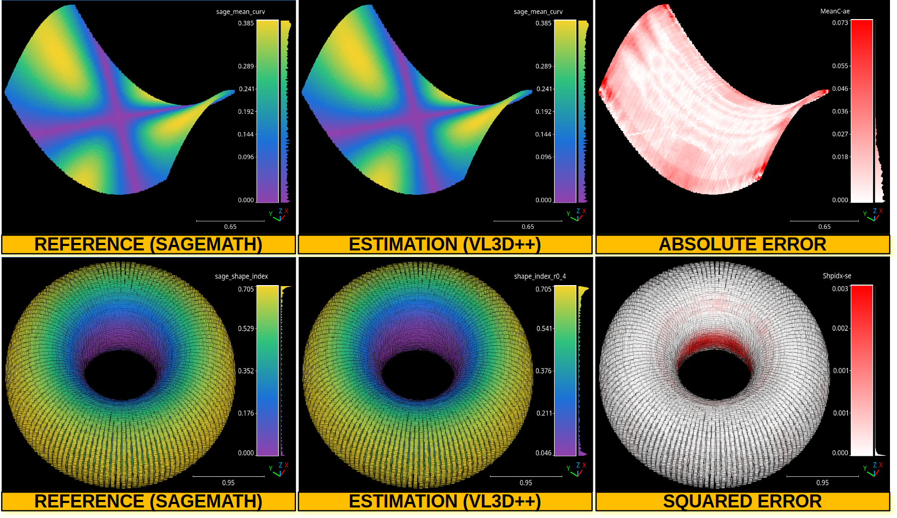
The top row shows the point-wise mean curvature and its absolute error on an hyperbolic paraboloid. The bottom row shows the point-wise shape index and its squared error on a torus.

Simple curve evaluator

The SimpleCurveEvaluator quantifies the geometric quality of the curves produced by the SimpleCurveExtractor (or any compatible source) with respect to a point cloud. It consumes the extractor’s output as an in-memory list of curve dicts (each entry carries the polyline vertices under 'points' and the per-feature metadata, including CURVE_ID). Inside a pipeline the channel is populated automatically by the upstream extractor and forwarded to the evaluator via the curves attribute of the pipeline state.. It reports five Key Performance Indicators (KPIs):

• Coverage \((\%)\) — fraction of curve-class input points whose closest extracted-curve point is within coverage_radius metres in 3D Euclidean distance.

• Deviation \((\%)\) — length-weighted ratio of extracted polyline 3D arc that traverses populated input regions but where no curve-class input point is nearby. A densified polyline vertex counts as deviating when no curve-class input neighbor lies within hallucination_radius (i.e. it is hallucinated) AND at least one any-class input neighbor lies within hallucination_radius (i.e. it sits inside the cloud). By construction \(\mathrm{Deviation} + \mathrm{PureHallucination} = \mathrm{Hallucination}\) segment-exact under the both/one segment-mask convention shared with the hallucination metric.

• Hallucination \((\%)\) — length-weighted ratio of extracted curve material whose densified vertices have no input curve-class support within hallucination_radius (3D). The evaluator also reports the count of features whose individual hallucination score exceeds hallucination_feature_threshold.

• Self-intersections — count of unordered pairs of 2D polyline-segment crossings that share the same CURVE_ID.

• Gaps — sum across CURVE_ID of feature-endpoint pairs from different features of the same curve whose 2D distance is in \((\varepsilon, r_{\mathrm{gap}}]\). T-junctions (endpoint sitting close to another feature’s interior vertex) can optionally be excluded.

Coverage, Deviation and Hallucination are 3D metrics (length-anchored for Deviation and Hallucination, point-anchored for Coverage); Self-intersections and Gaps are 2D, since they describe XY topology.

A SimpleCurveEvaluator can be defined inside a pipeline using the JSON below:

{
    "eval": "SimpleCurveEvaluator",
    "coverage_radius": 3.0,
    "deviation_radius": 2.0,
    "hallucination_radius": 2.5,
    "hallucination_feature_threshold": 0.025,
    "densify_step": 0.5,
    "gap_radius": 15.0,
    "gap_eps": 1e-6,
    "exclude_t_junctions": true,
    "t_radius": 5.0,
    "self_intersection_grid_cell": 5.0,
    "self_intersection_eps": 1e-6,
    "self_intersection_parallel_threshold": 1e-12,
    "degenerate_segment_length": 1e-12,
    "curve_class": 4,
    "report_path": "*report/simple_curve_eval.log",
    "hallucination_report_path": "*report/simple_curve_hall.csv",
    "summary_plot_path": "*plot/simple_curve_summary.png",
    "hallucination_plot_path": "*plot/simple_curve_hall.png"
}

The evaluator does not take a curves path because the extractor already exposes the polylines in memory. The SimpleCurveExtractor populates state.curves with a list of dicts (vertices under 'points' plus CURVE_ID and the rest of the per-feature metadata) and the pipeline executor forwards it to SimpleCurveEvaluator.eval() automatically. SHP/CSV/GPKG output writers continue to work in parallel and the in-memory channel is purely additive.

Arguments

– coverage_radius

Coverage neighborhood radius (m, 3D). A curve-class input point is considered COVERED when its 3D distance to any extracted-curve point is at most this value. Default 3.0.

– deviation_radius

Radius (m, 3D) used only by the n_isolated context KPI: an input curve-class point is flagged isolated when it has no other input neighbor within this radius. The length-anchored deviation_pct is computed at hallucination_radius and does not consult this value. Default 2.0. Note that deviation_radius only governs the n_isolated context KPI. The length-anchored deviation_pct is computed at hallucination_radius (see the Deviation bullet above).

– hallucination_radius

Hallucination neighborhood radius (m, 3D). A densified polyline vertex is hallucinated when no input curve-class point lies within this radius. Default 2.5.

– hallucination_feature_threshold

Per-feature hallucination score above which a feature is flagged as hallucinated. Default 0.025 (i.e. 2.5 %).

– densify_step

Polyline densification step (m, 3D arc). Coverage and Hallucination both reuse this densification. Default 0.5.

– gap_radius

Maximum endpoint-to-endpoint 2D distance for a candidate gap pair (m). Default 15.0.

– gap_eps

Endpoint distance below which a pair counts as touching, not as a gap. Default 1e-6.

– exclude_t_junctions

Whether to skip endpoint pairs where an endpoint sits within t_radius of the other feature’s interior vertices. Such pairs are legitimate branch points (T-junctions), not unclosed gaps. Default false.

– t_radius

Radius (m) for the T-junction test. Default 5.0.

– self_intersection_grid_cell

Cell size (m) of the bounding-box grid used by the self-intersection counter to localise candidate segment pairs. The grid turns the scan from \(O(N^{2})\) to \(O(N k)\). The value should be commensurate with the typical polyline segment length: too small wastes memory on empty cells, too large defeats the spatial pruning. This parameter is case-dependent — input geometries with very small or very large segment lengths need a matching cell size. Default 5.0.

– self_intersection_eps

Tolerance on the parametric-interval test that decides whether two 2D segments cross. Two segments are taken to cross when their parameters t and u both fall in \((-\varepsilon, 1+\varepsilon)\). Unitless on the parameter space. Default 1e-6.

– self_intersection_parallel_threshold

Magnitude of the cross-product below which the two direction vectors are treated as parallel and the crossing test short-circuits to False. Scales with the squared coordinate magnitudes, so very large or very small coordinate ranges may need a different value. Default 1e-12.

– degenerate_segment_length

3D segment lengths below this threshold are skipped during polyline densification (no intermediate points inserted), avoiding divide-by-zero and n_insert blow-ups on near-degenerate segments. Scales with the unit of the input coordinates. Default 1e-12.

– curve_class

Classification value identifying curve points in the input cloud. Default 4.

– report_path

Path to write the textual KPI report.

– hallucination_report_path

Path to write the per-feature hallucination CSV (feature_index,score,hall_len,feat_len).

– summary_plot_path

Path to write the KPI summary figure (Coverage, Deviation (length-anchored), Hallucination, count of hallucinated features, Self-intersections and Gaps).

– hallucination_plot_path

Path to write the per-feature hallucination histogram with a vertical reference line at hallucination_feature_threshold.

Output

The evaluator produces a textual report describing the five KPIs and the inputs context (curve-class point count, densified-vertex count, distinct CURVE_IDs), an optional per-feature hallucination CSV, and two figures: a KPI summary bar chart and a per-feature hallucination histogram. The report below corresponds to the example JSON:

     Simple curve evaluation report
==========================================

Inputs:
  Curve class:      4
  Curve points:     5770345
  Features:         135
  CURVE_IDs:        72
  Densified pts:    88448 (step=0.5 m, 3D)


Summary:
  Coverage:               88.3015 %
  Deviation (length 3D):  0.4765 %
  Isolated curve pts:     0
  Hallucination:          0.4922 %
  Hallucinated features:  9 / 135 (6.6667 %)
  Self-intersections:     0
  Gaps (total):           12
  T-junctions excluded:   66


Numerical settings:
  SI grid cell:             5 m
  SI parametric eps:        1e-06
  SI parallel threshold:    1e-12
  Degenerate seg length:    1e-12 m

Deep learning model evaluator

The DLModelEvaluator assumes there is a deep learning at the current pipeline’s state that can be used to process the point cloud at the current pipeline’s state. Instead of returning the output point-wise predictions, the values of the output layer and some internal feature representation will be returned to be visualized directly in the point cloud. Note that the internal feature representation might need an enormous amount of memory as it scales depending on how many features are generated by the architecture at the studied layer. A DLModelEvaluator can be defined inside a pipeline using the JSON below:

{
    "eval": "DLModelEvaluator",
    "pointwise_model_output_path": "pwise_out.las",
    "pointwise_model_activations_path": "pwise_activations.las"
}

The JSON above defines a DLModelEvaluator that will export the values of the output layer to the file pwise_out.las and a representation of the features in the hidden layers to the file pwise_activations.las.

Arguments

– pointwise_model_output_path

Where to export the point cloud with the point-wise outputs of the neural network.

– pointwise_model_activations_path

Where to export the point cloud with the internal features of the neural network.

Output

The output is illustrated considering the March 2018 point clouds from the Hessigheim dataset to compute the deep learning model evaluation. The figure below illustrates four different features extracted by the neural network. They are taken as the activated outputs of the last layer before the softmax .

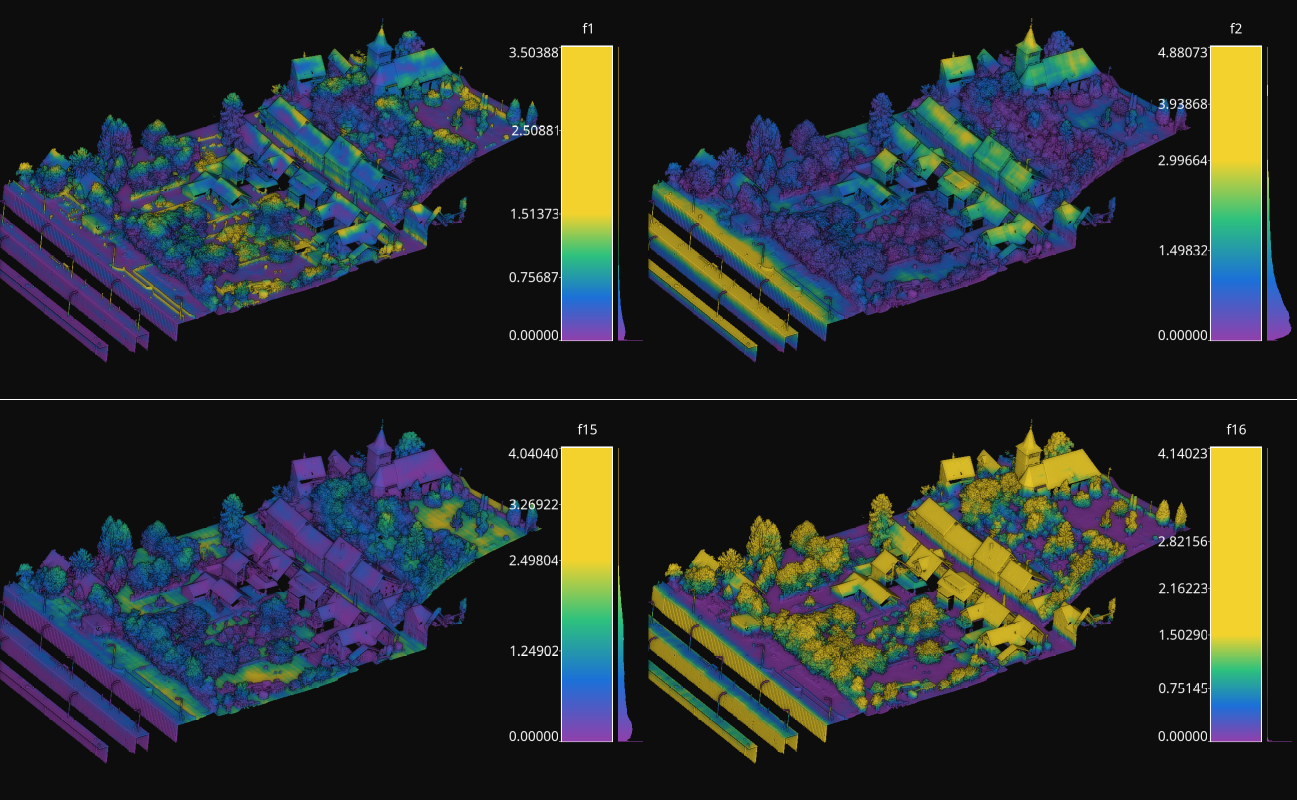
Visualization of some features used by a PointNet-based neural network for point-wise classification.

Raster grid evaluator

The RasterGridEvaluator can be used to evaluate the point cloud on a grid. This grid can later be exported to a GeoTIFF file that extends the grid with geographic information. Therefore, the GeoTIFF can be used to evaluate the features or classifications in the point cloud, e.g., loading the GeoTIFF in a GIS software to compare the rasterized point cloud with satellite image or maps in general. The GeoTIFFs are generated using the RasterIO library.

{
            "eval": "RasterGridEvaluator",
            "crs": "+proj=utm +zone=29 +ellps=GRS80 +towgs84=0,0,0,0,0,0,0 +units=m +no_defs +type=crs",
            "plot_path": "*geotiff/",
            "conditions": null,
            "xres": 1.0,
            "yres": 1.0,
            "grid_iter_step": 1024,
            "grids": [
                    {
                            "fnames": ["Vegetation"],
                            "reduce": "mean",
                            "empty_val": "nan",
                            "target_relational": "equals",
                            "oname": "vegetation_mean"
                    },
                    {
                            "fnames": ["Vegetation"],
                            "reduce": "max",
                            "empty_val": "nan",
                            "target_relational": "equals",
                            "oname": "vegetation_max"
                    },
                    {
                            "fnames": ["prediction"],
                            "target_val": 2,
                            "target_relational": "equals",
                            "reduce": "binary_mask",
                            "count_threshold": 3,
                            "empty_val": "nan",
                            "oname": "vegetation_mask"
                    },
                    {
                            "fnames": ["Ground", "Vegetation", "Other"],
                            "reduce": "mean",
                            "empty_val": "nan",
                            "target_relational": "equals",
                            "oname": "GVO_mean"
                    },
                    {
                            "fnames": ["Ground", "Vegetation", "Other"],
                            "reduce": "max",
                            "empty_val": "nan",
                            "target_relational": "equals",
                            "oname": "GVO_max"
                    },
                    {
                            "fnames": ["PointWiseEntropy"],
                            "reduce": "mean",
                            "empty_val": "nan",
                            "target_relational": "equals",
                            "oname": "pwise_entropy_mean"
                    },
                    {
                            "fnames": ["PointWiseEntropy"],
                            "reduce": "max",
                            "empty_val": "nan",
                            "target_relational": "equals",
                            "oname": "pwise_entropy_max"
                    }
            ]
    }

The JSON above defines a RasterGridEvaluator that generates many GeoTIFFs using the EPSG:25829 coordinate reference system (specified using PROJ syntax). The GeoTIFFs are exported to the geotiff subdirectory, considering the output prefix of the pipeline. The cell size is \(1\,\mathrm{m}\) along each axis. Some GeoTIFFs use a single color channel to represent a continuous value. One particular GeoTIFF generates a binary mask for each cell with \(1\) when there are at least \(3\) points classified as vegetation and \(0\) otherwise. The GeoTIFFs that consider the likelihood for Ground, Vegetation, and Other classes will export each likelihood in a different color channel.

Arguments

– crs

The coordinate reference system specification. See the RasterIO documentation for more information about CRS specification.

– plot_path

The directory where the GeoTIFF files will be stored.

– conditions

A list with many conditions specified as dictionaries. These conditions will be applied to filter the entire point cloud before computing any raster or grid. See the advanced evaluator conditions documentation for further details.

– xres

The cell resolution along the x-axis.

– yres

The cell resolution along the y-axis.

– grid_iter_step

How many max rows per iteration. It can be tuned to improve the efficiency but also to prevent memory exhaustion.

– radius_expr

An optional specification to define the computation of the radius for the ball-like neighborhoods. The variable "l" represents the max cell size and it is the default radius expression. Note that any expression less than "sqrt(2)*l/2" (half of the cell’s hypotenuse) will potentially ignore some points inside the cell boundary. Also, values greater than the previous one will increase the “smooth” effect through more overlapped neighborhoods.

– grids

A list with potentially many grid specifications. A grid can be specified with a dictionary-like style:

{
    "fnames": ["feat1", "feat2"],
    "reduce": "mean",
    "empty_val": "nan",
    "target_relational": "equals",
    "target_val": 2,
    "count_threshold": 3,
    "oname": "my_geotiff"
}

The fnames list must specify the name of the involved features. It can be null but only when the reduce strategy is "binary_mask" (binary occupation mask, i.e., whether a cell contains at least one point or not), "recount" (number of points per cell) or "relative_recount" (normalized number of points per cell).

The optional conditions list must specify the conditional filters that must be applied to the data for a particular grid. Its specification is the same as for the advanced evaluator conditions.

The reduce string must refer to a strategy to reduce many values per cell to a single one, e.g., "mean", "median", "min", "max", "binary_mask", "recount", and "relative_recount".

The empty_val value will be assigned to represent the cells with no points. They can be numbers or the string "nan" (not a number).

The target_relational governs how the values will be compared against the target. Supported relationals are "equals" (\(=\)), "not_equals" (\(\neq\)), "less_than" (\(<\)), "less_than_or_equal_to" (\(\leq\)), "greater_than" (\(>\)), "greater_than_or_equal_to" (\(\geq\)), "in" (\(\in\)), and "not_in" (\(\notin\)). Note that it must be given even if not used.

The target_val the value that must be searched when using a binary mask strategy.

The count_threshold governs how many times the target value must be found to consider a \(1\) for the binary mask.

The dem overloads the previous specifications and instead computes a Digital Elevation Model (DEM) assuming the \((x, y)\) plane with elevation values corresponding to \(z\). Note that since all the other arguments are ignored, only the global conditions of the RasterGridEvaluator are applied. Post-processing interpolations are still possible but generally not especially useful as the DEM already involves a 2D grid interpolation. The DEM is computed through the DEMGenerator class. It supports selecting its internal interpolation strategy (either "linear", "nearest", or "cubic"), by default it is

"dem": {
    "interpolation": "linear"
}

The interpolator can post-process the generated raster to interpolate some cells considering the values in the others through radial basis functions. It is based on the GridInterpolator2D class. Below an example of a potential interpolator specificaiton for a particular grid:

"interpolator": {
    "iterations": 2,
    "domain": {
        "strategy": "polygonal_contour_target",
        "channel": 0,
        "erosions": 2,
        "dilations": 3,
        "polygonal_approximation": 0,
        "target_val": "nan",
        "target_relational": "equals"
    },
    "interpolation": {
        "smoothing": 0.0,
        "kernel": "linear",
        "neighbors": 64,
        "epsilon": null,
        "degree": null,
        "clip_interval": [0, null]
    }
}

The arguments of the interpolator are:

– iterations

How many times apply the entire interpolation strategy to the grid.

– domain

The specification of the first stage where the cells that must be interpolated are determined. Its arguments are:

– strategy

The strategy to determine the cells to be interpolated. It can be: "all" to interpolate all the cells in the grid, "target" to interpolate only the cells in the grid that satisfy the given relational, "polygonal_contour" to interpolate all the cells in the grid inside the region closed by the contour of the cells that do not satisfy the given relational, or "polygonal_contour_target" to interpolate only the cells that satisfy the given relational and are inside the region closed by the contour of the cells that do not satisfy the given relational.

– channel

The channel (default 0) that must be selected when the grid contains many values per cell to check the relational.

– erosions

How many morphological erosions perform before computing the contour (see scikit-image documentation about erosion).

– dilations

How many morphological dilations perform after the erosions but before computing the contour (see scikit-image documentation about dilation).

– polygonal_approximation

The tolerance for the polygonal approximation using the Douglas-Peucker algorithm. Note that if zero is given there is no polygonal approximation at all. (see scikit-image documentation about approximate polygons).

– target_val

The target value for the relational check. Typically, it will be a number. However, it can be a list given the two endpoints of the interval for "inside_open" and "inside_close" relationals or a list representing the items of a set for "in" and "not_in" relationals.

– target_relational

The relational itself. It can be either "equals" (\(=\)), "not_equals" (\(\neq\)), "less_than" (\(<\)), "less_than_or_equal_to" (\(\leq\)), "greater_than" (\(>\)), "greater_than_or_equal_to" (\(\geq\)), "inside_open" (\(\in (a, b)\)), "inside_close" (\(\in [a, b]\)), "in" (\(\in\)), or "not_in" (\(\notin\)).

– interpolation

The specification of the second stage where the cells that must be interpolated are effectively interpolated.

– kernel

See the kernel parameter in the SciPy documentation.

– smoothing

See the smoothing parameter in the SciPy documentation.

– neighbors

See the neighbors parameter in the SciPy documentation.

– epsilon

See the epsilon parameter in the SciPy documentation.

– degree

See the degree parameter in the SciPy documentation.

– clip_interval

If given, it must be a list of exactly two elements. The first element is the min value such that any value in the grid that is below it will be set to the min value. The second element is the max value such that any value in the grid that is above it will be set to the max value. One of the elements in this list can be null. In that chase, no clipping to that endpoint will be applied.

The hillshading specification, as a post-processing step to improve the visibility of certain landforms in the output raster. Below an example of the hillshading post-processing with default values:

"hillshading": {
    "azimuth": 30,
    "altitude": 30
}

The arguments for the hillshading specification are:

– azimuth

The angle of the light source with respect to the surface. It must be inside \([0, 360)\) degrees.

—altitude The angle where the light source is located. It must be inside \([0, 90]\) degrees.

The oname name for the output GeoTIFF file corresponding to the grid specification.

– reverse_rows

Boolean flag to control whether to reverse the rows of the grid (True) or not (False). The default is the reversed order, i.e., True.

– nthreads

The number of threads for the parallel computation of the grids. By default, just one thread is used. The value -1 implies using as many threads as available cores.

Output

The output is illustrated considering some MLS points clouds acquired in the region of Pontevedra, Galicia, northwest Spain. The points sum up to \(6.15 \times 10^{8}\) from a dataset of \(3.51 \times 10^{9}\) points.

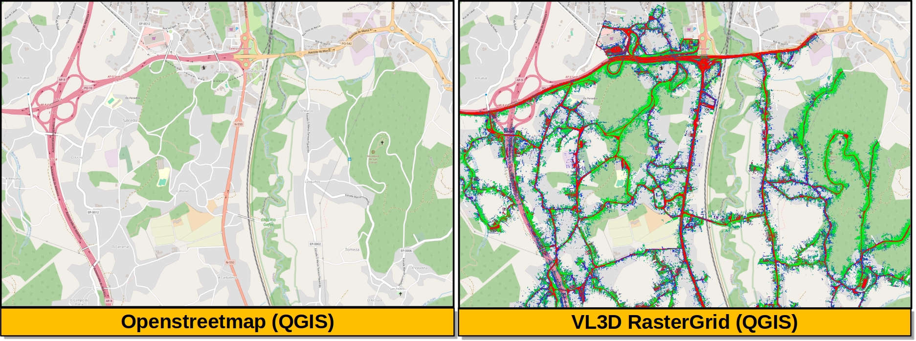
Visualization of the output GeoTIFFs on QGIS as an overlay to the Openstreetmap of the region of Pontevedra in Galicia, northwest Spain. The red color represents the mean ground likelihood in the neighborhood, green the vegetation likelihood, and blue any other class (e.g., buildings and powerlines).

Raster grid evaluator (PP)

The RasterGridEvaluatorPP is the C++/OpenMP-accelerated version of RasterGridEvaluator. It produces the same family of GeoTIFFs (reducer grids, DEM, binary masks, recounts, etc.) but offloads the per-cell sweep and the post-processing kernels to C++ code exposed by pyvl3dpp.

Legacy pipeline JSONs are largely drop-in compatible. In the common case it is enough to replace "eval": "RasterGridEvaluator" by "eval": "RasterGridEvaluatorPP" and the existing grids specifications keep working as they did. The intentional divergences documented below cover the few cases where the behavior of this version is deliberately stricter, more permissive, or numerically different from the python-based implementation.

On top of that, the PP evaluator adds five new per-grid post-processing kernels that operate directly on the rasterized \((x, y) \to z\) grid. A Horn-style hillshade, a local relief model (lrm), a SAGA/RVT-style resampling_filter, a visualization for archaeological topography (vat), and a multi-scale relief model (msrm). These can be combined with the existing dem and interpolator specifications to produce richer geomorphological visualizations from a single evaluator run.

{
    "eval": "RasterGridEvaluatorPP",
    "crs": "+proj=utm +zone=29 +ellps=GRS80 +towgs84=0,0,0,0,0,0,0 +units=m +no_defs +type=crs",
    "plot_path": "*geotiff/",
    "conditions": null,
    "xres": 1.0,
    "yres": 1.0,
    "grid_iter_step": 1024,
    "tree_type": "auto",
    "nthreads": -1,
    "grids": [
        {
            "dem": {"interpolation": "linear"},
            "empty_val": "nan",
            "oname": "dem"
        },
        {
            "fnames": ["Vegetation"],
            "reduce": "mean",
            "empty_val": "nan",
            "oname": "vegetation_mean"
        },
        {
            "fnames": ["prediction"],
            "target_val": 2,
            "target_relational": "equals",
            "reduce": "binary_mask",
            "count_threshold": 3,
            "empty_val": "nan",
            "oname": "vegetation_mask"
        },
        {
            "dem": {"interpolation": "linear"},
            "empty_val": "nan",
            "hillshade": {
                "azimuth": 315,
                "altitude": 45,
                "z_factor": 1.0
            },
            "oname": "dem_hillshade"
        },
        {
            "dem": {"interpolation": "linear"},
            "empty_val": "nan",
            "lrm": {
                "radius": 5,
                "filter": "mean",
                "edge_mode": "reflect"
            },
            "oname": "dem_lrm"
        },
        {
            "dem": {"interpolation": "linear"},
            "empty_val": "nan",
            "msrm": {
                "fmin": 1.0,
                "fmax": 25.0,
                "x": 2.0,
                "edge_mode": "reflect"
            },
            "oname": "dem_msrm"
        },
        {
            "dem": {"interpolation": "linear"},
            "empty_val": "nan",
            "vat": {
                "hillshade": {
                    "azimuth": 315,
                    "altitude": 45,
                    "z_factor": 1.0
                },
                "n_directions": 16,
                "search_radius": 20,
                "svf_opacity": 0.5,
                "po_opacity": 0.5
            },
            "oname": "dem_vat"
        }
    ]
}

The JSON above defines a RasterGridEvaluatorPP that generates several GeoTIFFs using the EPSG:25829 coordinate reference system (specified using PROJ syntax). The cell size is \(1\,\mathrm{m}\) along each axis. The pipeline produces a DEM, a per-cell vegetation likelihood mean, a binary occupation mask of vegetation predictions, and four new derived rasters computed from the DEM: 1) Horn hillshade, 2) local relief model, 3) multi-scale relief model, and 4) VAT composite.

Arguments

Only the new top-level arguments and the changed defaults are listed below. The shared arguments crs, plot_path, conditions, xres, yres, grid_iter_step, radius_expr, nthreads, and grids are documented under RasterGridEvaluator and keep the same semantics.

– tree_type

Selector forwarded to the C++ NeighborhoodComputer to choose the spatial index used by the cylinder neighborhood queries. "auto" (the default) lets the C++ side pick the best tree given the input size and is the recommended setting.

– nthreads

Number of OpenMP threads used by the C++ sweep and the post-processing kernels. The default is \(-1\) (use all available threads). This differs from the legacy default (\(1\)); see the divergences subsection above.

– reverse_rows

Boolean flag kept for legacy JSON compatibility. It is currently a no-op: the PP evaluator always writes rows in the same order as the legacy evaluator with reverse_rows = True (see raster_grid_evaluator.py lines 264-266), which is the GeoTIFF-friendly orientation.

New per-grid keys

In addition to the legacy per-grid keys (dem, hillshading, interpolator, etc.) the PP evaluator accepts five new keys that post-process the rasterized grid. They are designed for DEM-like grids but can be applied to any 2D raster produced by an upstream reducer.

Hillshade (Horn)

Horn’s algorithm uses a \(3 \times 3\) Sobel-like stencil to estimate the surface gradient at each cell:

\[g_x = \frac{1}{8\,x_{\mathrm{res}}} \big((c+2f+i) - (a+2d+g)\big),\quad g_y = \frac{1}{8\,y_{\mathrm{res}}} \big((g+2h+i) - (a+2b+c)\big),\]

with \(a,\ldots,i\) the nine neighbors of the centre cell in row-major order. The slope and aspect follow from

\[\mathrm{slope} = \arctan\!\big(z_f\,\sqrt{g_x^2 + g_y^2}\big),\quad \mathrm{aspect} = \mathrm{atan2}(g_y,\, -g_x),\]

where \(z_f\) is the z_factor argument. The solar zenith and math-CCW azimuth are obtained from the user-facing angles via \(\mathrm{zen} = (90 - \mathrm{alt})\,\pi/180\) and \(\mathrm{azm}_{\mathrm{ccw}} = (360 - \mathrm{az} + 90)\,\pi/180\), and the final cell intensity is

\[\mathrm{hs} = \mathrm{clip}\!\big( \cos(\mathrm{zen})\,\cos(\mathrm{slope}) + \sin(\mathrm{zen})\,\sin(\mathrm{slope}) \,\cos(\mathrm{azm}_{\mathrm{ccw}} - \mathrm{aspect}), \;0,\;1\big).\]

The defaults are azimuth = 315, altitude = 45, and z_factor = 1.0, matching the GDAL convention. See Horn (1981, “Hill shading and the reflectance map”, Proceedings of the IEEE and gdaldem hillshade -alg Horn.

"hillshade": {
    "azimuth": 315,
    "altitude": 45,
    "z_factor": 1.0
}

Local Relief Model (LRM)

The LRM exposes small-scale topographic variability by subtracting a low-pass version of the input grid from itself:

\[\mathrm{LRM}(p) = z_{\mathrm{2D}}(p) - \mathrm{lowpass}\!\big(z_{\mathrm{2D}},\; r_{\mathrm{cells}},\; \mathrm{edge\_mode}\big)(p),\]

where the low-pass is by default a NaN-aware box mean over a \((2r+1) \times (2r+1)\) window. The defaults are radius = 5 (cells), filter = "mean", and edge_mode = "reflect". The edge_mode argument can also be "nearest". See Hesse (2010, “LiDAR-derived local relief models - a new tool for archaeological prospection”, Archaeological Prospection) .

"lrm": {
    "radius": 5,
    "filter": "mean",
    "edge_mode": "reflect"
}

Resampling filter

The resampling filter smooths the raster by aggregating it to a coarser grid and then bicubically interpolating back to the original cell size. The aggregation step is NaN-aware and area-weighted. Each coarse cell is the mean of the finite values inside a scale_factor \(\times\) scale_factor window. The up-sample step uses scipy.interpolate.RectBivariateSpline() with kx=3, ky=3, and s=0 (see Intentional divergences from RasterGridEvaluator ). The default is scale_factor = 10.

"resampling_filter": {
    "scale_factor": 10
}

Visualization for Archaeological Topography (VAT)

VAT composes four classic relief visualizations into a single grayscale layer that emphasizes archaeological microtopography: hillshade, slope, positive openness (PO), and sky-view factor (SVF). The four layers are blended by an overlay of hillshade with slope, then a screen with positive openness, then a multiply with the sky-view factor:

\[\begin{split}\mathrm{VAT}_0 &= \mathrm{overlay}(\mathrm{HS},\,\mathrm{slope}),\\ \mathrm{VAT}_1 &= \mathrm{screen}(\mathrm{VAT}_0,\,\mathrm{PO};\, \alpha_{\mathrm{po}}),\\ \mathrm{VAT} &= \mathrm{multiply}(\mathrm{VAT}_1,\,\mathrm{SVF};\, \alpha_{\mathrm{svf}}).\end{split}\]

The defaults are hillshade.azimuth = 315, hillshade.altitude = 45, hillshade.z_factor = 1.0, n_directions = 16, search_radius = 20 (cells), svf_opacity = 0.5, and po_opacity = 0.5. See Kokalj and Somrak (2019, “Why not a single image? Combining visualizations to facilitate fieldwork and on-screen mapping”, Remote Sensing) .

"vat": {
    "hillshade": {
        "azimuth": 315,
        "altitude": 45,
        "z_factor": 1.0
    },
    "n_directions": 16,
    "search_radius": 20,
    "svf_opacity": 0.5,
    "po_opacity": 0.5
}

Multi-Scale Relief Model (MSRM)

The MSRM aggregates several scale-specific relief models into a single raster. With \(r_r = (|x_{\mathrm{res}}| + |y_{\mathrm{res}}|)/2\) the average cell size, the scale range is derived from the user-supplied minimum and maximum feature sizes fmin and fmax and the exponent x via

\[\begin{split}i &= \left\lfloor \left(\frac{\max(f_{\min},\, r_r) - r_r} {2\,r_r}\right)^{1/x}\right\rfloor,\\ n &= \left\lceil \left(\frac{f_{\max} - r_r}{2\,r_r}\right)^{1/x}\right\rceil.\end{split}\]

For each integer scale \(k \in [i,\,n]\) the corresponding low-pass grid is \(\mathrm{LP}_k = \mathrm{boxmean}(z_{\mathrm{2D}},\, \mathrm{round}(k^{\,x}),\, \mathrm{edge\_mode})\), the per-scale relief model is \(\mathrm{RM}_k = \mathrm{LP}_k - \mathrm{LP}_{k+1}\) for \(k \in [i,\,n-1]\), and the final raster is

\[\mathrm{MSRM} = \frac{1}{n-i} \sum_{k=i}^{n-1} \mathrm{RM}_k.\]

The defaults are x = 2.0 and edge_mode = "reflect"; fmin and fmax are mandatory and must satisfy \(f_{\max} > f_{\min} > 0\). See Orengo and Petrie (2018, “Multi-scale relief model (MSRM): a new algorithm for the visualization of subtle topographic change of variable size in digital elevation models”, Earth Surface Processes and Landforms) .

"msrm": {
    "fmin": 1.0,
    "fmax": 25.0,
    "x": 2.0,
    "edge_mode": "reflect"
}

Intentional divergences from RasterGridEvaluator

The C++ evaluator is compatible with the python one for the overwhelming majority of grid specifications. The following items are the only known intentional divergences.

– Hillshading uses Horn (not earthpy)

The hillshading post-processor dispatches to a C++ Horn implementation that follows the gdaldem hillshade -alg Horn convention (see cpp/include/raster/RasterPostProcessors.hpp). The legacy JSON parameter names and defaults (azimuth=30, altitude=30) are preserved at the JSON layer for drop-in compatibility, but the numerical output differs from earthpy.spatial.hillshade. Pipelines that persist legacy hillshade GeoTIFFs as ground truth will observe a numerical shift when migrating to the C++ evaluator.

– target_relational relaxed for arithmetic reducers

Grids that use the reducers mean, median, min, or max may omit the target_relational key. The C++ evaluator accepts those specifications because the relational is not consumed by those reducers. The legacy evaluator raises an EvaluatorException in that case. The C++ evaluator still raises an exception ('RasterGridEvaluatorPP failed because no target relational specification was given.') for the six reducers that actually consume the relational: binary_mask, binary_mask_nofeats, recount, recount_nofeats, relative_recount, and relative_recount_nofeats.

– Resampling-filter up-sample is Python-side

The resampling_filter post-processor splits the work between C++ and Python by design. The C++ kernel returns only the NaN-aware area-weighted coarse grid, and the bicubic up-sample to the original cell size is performed via scipy.interpolate.RectBivariateSpline() with kx=3, ky=3, and s=0. The split was chosen to keep the C++ side free of spline state while still recovering the original resolution at the GeoTIFF layer.

– Default nthreads = -1

The PP evaluator defaults to all OpenMP threads available on the host (nthreads=-1). The python evaluator defaults to a single thread.