Transformers

Transformers are components that apply a transformation on the point cloud. They can be divided into class transformers (ClassTransformer) that transform the classification and predictions of the point cloud, feature transformers (FeatureTransformer) that transform the features of the point cloud, and point transformers (PointTransformers) that compute an advanced transformation on the point cloud that involves different information (e.g., spatial coordinates to derive receptive fields that can be used to reduce or propagate both features and classes).

Transformers are typically use inside pipelines to apply transformations to the point cloud at the current pipeline’s state. Readers are strongly encouraged to read the Pipelines documentation before looking further into transformers.

Class transformers

Class reducer

The ClassReducer takes an original set of \(n_I\) input classes and returns \(n_O\) output classes, where \(n_O < n_I\). It can be applied to the reference classification only or also to the predictions. On top of that, it supports a text report on the distributions with the absolute and relative frequencies and a plot of the class distribution before and after the transformation. A ClassReducer can be defined inside a pipeline using the JSON below:

{
        "class_transformer": "ClassReducer",
        "on_predictions": false,
        "input_class_names": ["noclass", "ground", "vegetation", "cars", "trucks", "powerlines", "fences", "poles", "buildings"],
        "output_class_names": ["noclass", "ground", "vegetation", "buildings", "objects"],
        "class_groups": [["noclass"], ["ground"], ["vegetation"], ["buildings"], ["cars", "trucks", "powerlines", "fences", "poles"]],
        "report_path": "class_reduction.log",
        "plot_path": "class_reduction.svg"
}

The JSON above defines a ClassReducer that will replace the nine original classes into five reduced classes where many classes are grouped together as the "objects" class. Moreover, it will generate a text report in a file called class_reduction.log and a figure representing the class distribution in class_reduction.svg.

Arguments

– on_predictions

Whether to also reduce the predictions if any (True) or not (False). Note that setting on_predictions to True will only work if there are available predictions.

– input_class_names

A list with the names of the input classes.

– output_class_names

A list with the desired names for the output classes.

– class_groups

A list of lists such that the list i defines which classes will be considered to obtain the reduced class i. In other words, each sublist contains the strings representing the names of the input classes that must be mapped to the output class.

– report_path

Path where the text report on the class distributions must be written. If it is not given, then no report will be generated.

– plot_path

Path where the plot of the class distributions must be written. If it is not given, then no plot will be generated.

Output

The examples in this section come from applying a ClassReducer to the 5080_54435.laz point cloud of the DALES dataset .

An example of the plot representing how the classes are distributed before and after the ClassReducer is shown below.

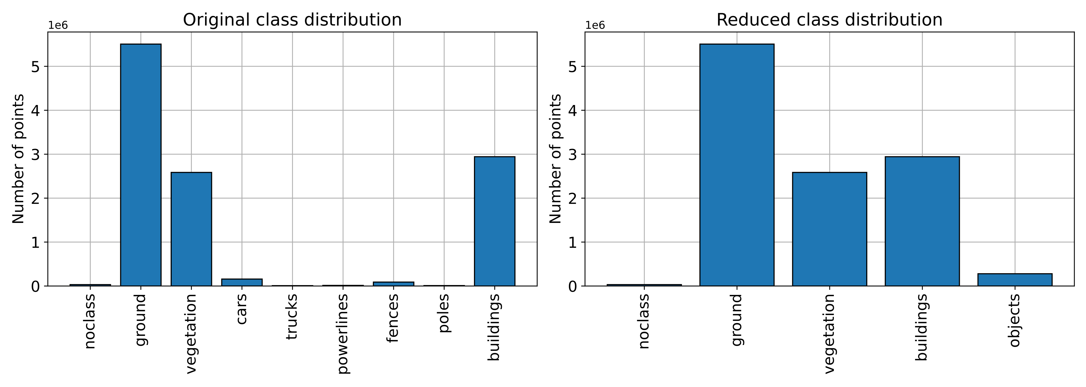
Visualization of the class distributions before and after the class reduction.

An example of how the classes represented on the point cloud look like before and after the ClassReducer is shown below.

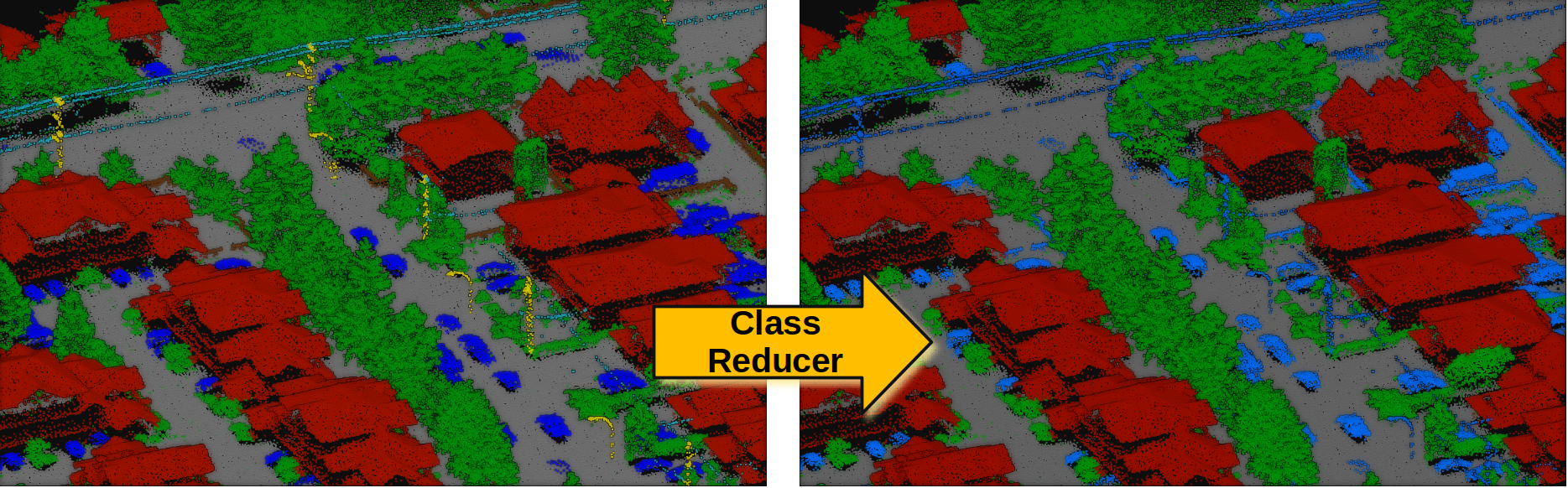
Visualization of the original (left) and reduced classification (right).

Class setter

The ClassSetter assigns the classes of a point cloud from any of its attributes. A ClassSetter can be defined inside a pipeline using the JSON below:

{
    "class_transformer": "ClassSetter",
    "fname": "prediction"
}

The JSON above defines a ClassSetter that will assign the "prediction" attribute as the point-wise classes of the point cloud.

Arguments

– fname

The name of the attribute that must be considered as the new classification of the point cloud.

Distance reclassifier

The DistanceReclassifier takes an original set of \(n_I\) input classes and returns \(n_O\) output classes. It can be applied to the reference classification or to the predictions. The transformation is based on relational filters, k-nearest neighbors neighborhoods, and point-wise distances involving the structure and feature spaces. It also supports a text report on the distributions with the absolute and relative frequencies and a plot of the class distribution before and after the transformation. A DistanceReclassifier can be defined inside a pipeline using the JSON below:

{
    "class_transformer": "DistanceReclassifier",
    "on_predictions": false,
    "input_class_names": ["ground", "vegetation", "building", "other"],
    "output_class_names": ["ground", "lowveg", "midveg", "highveg", "building", "other"],
    "reclassifications": [
      {
        "source_classes": ["vegetation"],
        "target_class": "highveg",
        "conditions": null,
        "distance_filters": null
      },
      {
        "source_classes": ["vegetation"],
        "target_class": "lowveg",
        "conditions": [
          {
            "value_name": "floor_dist",
            "condition_type": "less_than",
            "value_target": 0.5,
            "action": "preserve"
          }
        ],
        "distance_filters": null
      },
      {
        "source_classes": ["vegetation"],
        "target_class": "lowveg",
        "conditions": null,
        "distance_filters": [
          {
            "metric": "euclidean",
            "components": ["z"],
            "knn": {
              "coordinates": ["x", "y"],
              "max_distance": null,
              "k": 1,
              "source_classes": ["ground"]
            },
            "filter_type": "less_than",
            "filter_target": 1.0,
            "action": "preserve"
          }
        ]
      },
      {
        "source_classes": ["vegetation"],
        "target_class": "midveg",
        "conditions": null,
        "distance_filters": [
          {
            "metric": "euclidean",
            "components": ["z"],
            "knn": {
              "coordinates": ["x", "y"],
              "max_distance": null,
              "k": 1,
              "source_classes": ["ground"]
            },
            "filter_type": "inside",
            "filter_target": [1.0, 5.0],
            "action": "preserve"
          }
        ]
      }
    ],
    "report_path": "reclassification.log",
    "plot_path": "reclassification.svg",
    "nthreads": -1
}

The JSON above defines a DistanceReclassifier that will preserve the ground, building, and other classes while transforming the vegetation class into lowveg (low vegetation), midveg (mid vegetation), and highveg (high vegetation). In the process, it will generate a text report in a file called reclassification.log and a figure representing the class distributions in reclassification.svg.

Arguments

– on_predictions

Whether to also reduce the predictions if any (True) or not (False). Note that setting on_predictions to True will only work if there are available predictions.

– input_class_names

A list with the names of the input classes.

– output_class_names

A list with the desired names for the output/transformed classes.

– reclassifications

A list of dictionaries such that each dictionary specifies a class transform operation.

– source_classes

The names of the classes such that only points of these classes will be modified by the reclassification operation.

– target_class

The name of the target/output class to which those points that satisfy the conditions and distance-based filters will be assigned.

– conditions

A list of dictionaries such that each dictionary specifies a relational filter. See documentation about advanced input conditions .

– value_name

See documentation about advanced input conditions value name .

– condition_type

See documentation about advanced input condition type .

– value_target

See documentation about advanced input conditions value target .

– action

See documentation about advanced input conditions action .

– distance_filters

A list of dictionaries where each dictionary specifies a distance-based filter.

– metric

The distance metric to be computed for \(n\) components. It can be either "euclidean"

\[\operatorname{d}(\pmb{p}, \pmb{q}) = \sqrt{\sum_{j=1}^{n}{(p_j-q_j)^2}}\]

or "manhattan"

\[\operatorname{d}(\pmb{p}, \pmb{q}) = \sum_{j=1}^{n}{\left\lvert{p_j-q_j}\right\rvert} .\]

– components

A list with the names of the components defining the vectors whose distance will be computed. Supported components are "x", "y", and "z" for the corresponding coordinates from the structure space and also any feature name from the point cloud’s feature space.

– knn

The dictionary with the k-nearest neighbor neighborhood specification.

– coordinates

The coordinates defining the points for the neighborhood computations. For example, ["x", "y", "z"] implies typical 3D neighborhoods and ["x", "y"] implies typical 2D neighborhoods.

– max_distance

The max distance that any neighbor must satisfy. Points further away than this distance will be excluded from the neighborhood.

– k

The number of \(k\)-nearest neighbors.

– source_classes

Neighborhoods will only contain points belonging to the given source classes. If None, then all points will be considered as neighbors, no matter their class.

– filter_type

Like the advanced input condition type specification but also supports "inside" (\(x \in [a, b] \subset \mathbb{R}\)).

– filter_target

See documentation about advanced input conditions value target .

– action

See documentation about advanced input conditinos action .

– report_path

Path where the text report on the class distributions must be written. If it is not given, then no report will be generated.

– plot_path

Path where the plot of the class distributions must be written. If it is not given, then no plot will be generated.

– nthreads

The number of threads for the parallel computations. Note that using -1 means as many threads as available cores.

Output

The examples in this section come from applying a DistanceReclassifier to the PNOA_2015_GAL-W_478-4766_ORT-CLA-COL point cloud of the PNOA-II dataset .

The figure below is the plot representing how the classes are distributed before and after the DistanceReclassfier.

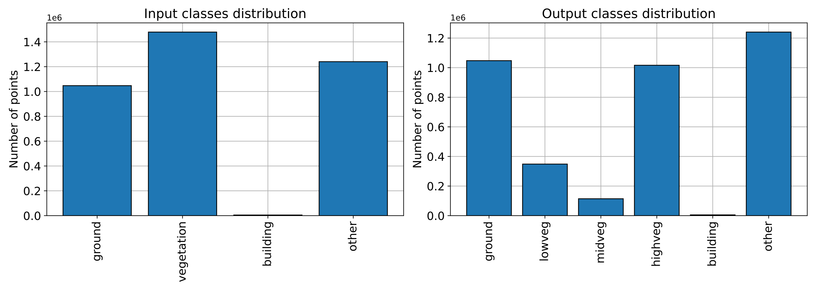
Visualization of the class distributions before and after the distance-based reclassification.

The figure below represents the vegetation reclassified by heights following the specifications from the JSON above (note that the floor distance was computed using the height features miner ++).

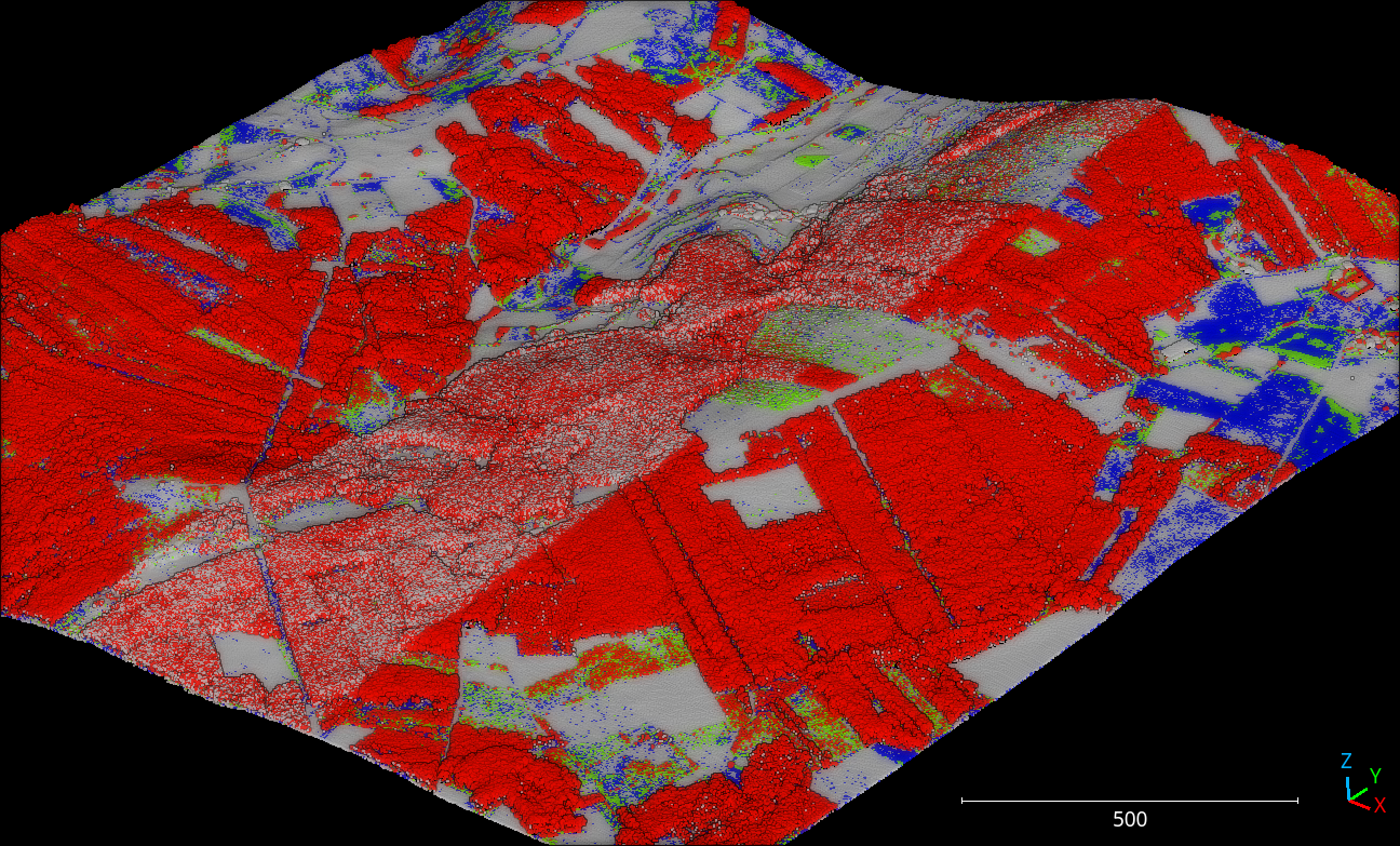
Visualization of the reclassified point cloud. Non-vegetation classes are colored white, low vegetation points are blue, mid vegetation ones are green, and high vegetation is red.

Directional reclassifier

The DirectionalReclassifier takes an original set of \(n_I\) input classes and returns \(n_O\) output classes. It can be applied to the reference classification or to the predictions. The transformation relabels points in user-specified source classes as overhang or underhang with respect to a locally fitted surface model. Each reclassifiable seed in a covering min-distance subsample grows a cluster via region growing, with the growth itself gated by PCA (the cluster is accepted while the smallest eigenvalue \(\lambda_{3}\) of its centered covariance stays at or below \(\tau^{2}\), where \(\tau\) is eigenthreshold). The local PCA frame \((\pmb{e}_{1}, \pmb{e}_{2}, \pmb{n})\) defines the \((u, v, h)\) coordinates in which the surface model is represented. For degree = 1 (default) the PCA plane itself is the surface model and the deviation thresholded against variety_distance_tolerance is the literal signed plane distance. For degree = 2 ... 5 a local polynomial \(h = \pmb{\theta}^{\intercal} \pmb{\phi}(u, v)\) (quadric, cubic, quartic, quintic) is solved by OLS (not PCA) in that frame, and an AICc model-selection step picks per cluster between the polynomial and its lower-degree truncations. Like DistanceReclassifier it supports a text report with the distributions before and after the transformation and a plot of those distributions. A DirectionalReclassifier can be defined inside a pipeline using the JSON below:

{
    "class_transformer": "DirectionalReclassifier",
    "on_predictions": true,
    "input_class_names": ["ground", "wall", "vegetation", "other", "break", "unlabeled"],
    "output_class_names": ["ground", "ground_obstacle", "wall", "wall_overhang", "wall_underhang", "vegetation", "other", "break", "unlabeled"],
    "reclassifications": [
        {
            "source_classes": ["wall"],
            "source_is_prediction": true,
            "forward_direction": [0, 0, 1],
            "target_overhang_class": "wall_overhang",
            "target_underhang_class": "wall_underhang",
            "conditions": [
                {
                    "value_name": "classification",
                    "condition_type": "equals",
                    "value_target": 1,
                    "action": "preserve"
                }
            ],
            "variety_distance_tolerance": 0.1,
            "eigenthreshold": 0.3,
            "init_radius": 5.0,
            "step_radius": 1.0,
            "min_distance": 0.1,
            "degree": 5,
            "trimmed_refit": true,
            "trim_factor": 1.0
        },
        {
            "source_classes": ["ground", "break"],
            "source_is_prediction": false,
            "forward_direction": [0, 0, 1],
            "target_overhang_class": "ground_obstacle",
            "target_underhang_class": null,
            "conditions": [
                {
                    "value_name": "classification",
                    "condition_type": "in",
                    "value_target": [0, 4],
                    "action": "preserve"
                }
            ],
            "variety_distance_tolerance": 0.1,
            "eigenthreshold": 0.033,
            "init_radius": 2.0,
            "step_radius": 1.0,
            "min_distance": 0.5,
            "degree": 2,
            "trimmed_refit": false,
            "trim_factor": 1.0
        }
    ],
    "report_path": "directional_reclassification.log",
    "plot_path": "directional_reclassification.svg",
    "nthreads": -1
}

The output feature columns (variety_distance, eigenmin, fit_quality, reclassification_cluster, reclassification_cluster_radius) are configured per reclassification entry, not at the top level. Add the corresponding *_as_feature and (optionally) *_name keys to whichever entries should produce that column. Each enabled column’s name must be unique across every reclassification — the validator at instantiation rejects collisions. With multiple reclassifications you typically pick distinct names (e.g. "wall_variety_distance" and "ground_variety_distance") so the LAS columns don’t collide.

The JSON above defines a DirectionalReclassifier that splits the "wall" class into core wall plus "wall_overhang" (points pulled forward of the local wall surface) and "wall_underhang" (points pushed backward of the wall surface), and tags ground points that protrude above the local ground plane as "ground_obstacle" while leaving any below-ground points unchanged (target_underhang_class is null). It will also generate a text report at directional_reclassification.log and a plot of the class distributions at directional_reclassification.svg.

The first reclassification entry uses "min_distance": 0.0 (the default) so the wall split runs directly on the input cloud. The second entry demonstrates the optional decimation path: "min_distance": 0.5 first subsamples the input via MinDistanceSubsampler at a 0.5 m radius, runs the region-growing PCA on that decimated representation only, and then propagates labels (and signed variety-distances when variety_distance_as_feature is true) to non-decimated source-class points by inheriting from each one’s closest decimated neighbor. This is useful for very dense clouds where running the algorithm on every point is wasteful.

The reclassification logic. Let \(P \subset \mathbb{R}^{3}\) be the set of points selected by the conditions filter (the geometric-computation set; defaults to the full cloud when no conditions are given) and let \(C \subset \mathbb{R}^{3}\) be the points whose class belongs to source_classes (the reclassifiable set). The algorithm picks covering seeds via min-distance subsampling on \(C \cap P\) at min_distance = init_radius and processes them in parallel. For each seed \(\pmb{q}\) it builds an initial neighborhood \(N(\pmb{q}) = \left\{\pmb{p} \in P : \lVert\pmb{p} - \pmb{q}\rVert \leq r_0\right\}\), which is always accepted, and then iteratively expands the cluster to \(\widetilde{N}(\pmb{q}) = N(\pmb{q}) \cup \left\{\pmb{p} \in P : \lVert\pmb{p} - \widetilde{\pmb{p}}\rVert \leq r_{\Delta}, \widetilde{\pmb{p}} \in \widetilde{P}\right\}\) where \(\widetilde{P}\) is the current frontier (newly-added cluster points belonging to \(C\)). The expansion is accepted only when \(\lambda_3(\widetilde{N}) \leq \tau^{2}\), where \(\lambda_3\) is the smallest eigenvalue of the centered covariance matrix of the cluster. Note that this gate is purely a cluster-shape constraint: it bounds how far a cluster may grow before the local covariance is no longer well-approximated as planar. For degree = 1 this gate doubles as the surface-model fit-quality threshold (since the PCA plane is the model); for degree 2..``5`` the polynomial fit is independent of \(\lambda_3\) and is solved by OLS only after the cluster has stopped growing. Its quality is assessed separately, by the AICc model-selection step (see the degree argument below). Reclassification at degree = 1 uses the centroid \(\pmb{\mu}\) and the smallest-eigenvalue eigenvector \(\pmb{n}\) of the last accepted state, sign-aligned with the user-supplied forward direction \(\pmb{u}\) (so \(\pmb{u}^{\intercal} \pmb{n} > 0\)):

\[\begin{split}\begin{aligned} (\pmb{x} - \pmb{\mu})^{\intercal} \pmb{n} \geq +\epsilon &\;\Rightarrow\; \text{overhang} \\ (\pmb{x} - \pmb{\mu})^{\intercal} \pmb{n} \leq -\epsilon &\;\Rightarrow\; \text{underhang} \\ \text{otherwise} &\;\Rightarrow\; \text{unchanged} \end{aligned}\end{split}\]

For degree 2..``5`` the same threshold semantics \(|d| \geq \epsilon \;\Rightarrow\; \text{label}\) apply, but \(d\) is replaced by a safeguarded geometric-distance estimate to the locally-fit polynomial surface (option-1 tangent-plane distance plus a one-step Newton refinement, with magnitude clamping); see the degree argument below for the full derivation.

When several regions claim the same point (overlap between covering seeds), the case with the largest neighborhood radius \(R(\pmb{q}) = \max_{\pmb{x} \in N(\pmb{q})} \lVert \pmb{x} - \pmb{\mu} \rVert\) wins. On equal radii, the seed with the smallest seed-id wins (deterministic across thread counts). Points in \(C\) that are not in \(P\) (e.g., source-class points filtered out by conditions) cannot seed regions and never appear in any neighborhood, so they are silently left unchanged.

Arguments

– on_predictions

Whether to also reclassify the predictions if any (True) or not (False). Note that setting on_predictions to True will only work if predictions are available.

– input_class_names

A list with the names of the input classes.

– output_class_names

A list with the desired names for the output/transformed classes.

– reclassifications

A list of dictionaries such that each dictionary specifies a directional reclassification operation.

– source_classes

The names of the classes such that only points of these classes will be modified by the reclassification operation. Note that, by default, all points are considered for the geometric computations; only those corresponding to source_classes will be modified. To consider in the computations only the source_classes, they must also be specified in conditions.

– source_is_prediction

Whether the source_classes must be taken from the "classification" attribute (False, the default) or from the "prediction" attribute (True).

– forward_direction

A three-component vector representing the forward direction. It is used to break the sign ambiguity of the estimated normal for the fitted plane. Internally normalized to unit length. Vectors with Euclidean norm below \(10^{-7}\) are rejected with an informative error.

– target_overhang_class

The name of the output class to assign to overhang points. When null, no overhang reclassification is performed.

– target_underhang_class

The name of the output class to assign to underhang points. When null, no underhang reclassification is performed.

– conditions

A list of dictionaries such that each dictionary specifies a relational filter. See documentation about advanced input conditions . When null or missing, the geometric-computation set \(P\) is the full cloud.

– value_name

See documentation about advanced input conditions value name . Additionally accepts "classification" and "prediction" to filter on the corresponding point-wise channel.

– condition_type

See documentation about advanced input condition type .

– value_target

See documentation about advanced input conditions value target .

– action

See documentation about advanced input conditions action .

– variety_distance_tolerance

The variety-distance tolerance \(\epsilon \geq 0\). Points whose signed projection on the local plane normal is at least \(+\epsilon\) are labeled as overhang; points with projection at most \(-\epsilon\) are labeled as underhang. Otherwise the class is left unchanged.

– eigenthreshold

The eigenvalue threshold \(\tau \geq 0\). A region-growing iteration is accepted when \(\lambda_3(\widetilde{N}) \leq \tau^{2}\), where \(\lambda_3\) is the smallest eigenvalue of the centered covariance of the trial cluster. The initial cluster (the one computed with init_radius) is always accepted regardless of \(\lambda_3\).

This gate is applied identically for every value of degree: it is a constraint on the cluster’s geometric shape (how close to planar the cluster’s PCA covariance is), not a constraint on the polynomial fit’s residuals. For degree = 1 it doubles as the surface-model fit-quality threshold (since the PCA plane is the model). For degree 2..``5`` the polynomial fit happens after cluster growth has finished, on the cluster the gate produced; its goodness-of-fit is measured by AICc on the residual sums of squares, not by \(\lambda_3\). Lowering eigenthreshold therefore tightens cluster shape (smaller, more strictly planar regions) regardless of the polynomial order, it does not, by itself, force a tighter polynomial fit on a curved cluster.

– init_radius

The initial sphere radius \(r_0 > 0\) for the seed query. Also used as the minimum distance for the covering subsampling of seeds, so every reclassifiable point is within \(r_0\) of at least one seed.

– step_radius

The expansion radius \(r_{\Delta} > 0\) for each region-growing iteration around the current frontier.

– min_distance

Optional min-distance decimation radius \(d_{*} \geq 0\). When > 0, the input cloud is first subsampled via MinDistanceSubsampler at this radius, the region-growing PCA runs on the decimated representation, and every point in the reclassification domain (i.e., source-class point) that was NOT kept by the decimation inherits its label (and signed variety-distance, when variety_distance_as_feature is true) from its closest decimated neighbor. When 0 (the default), null, or missing, no decimation is applied and the algorithm runs directly on the input cloud. The iter-1..iter-5 behavior is preserved bit-for-bit.

– degree

Order of the local surface model fit to each cluster. Defaults to 1. Supported values are 1, 2, 3, 4, and 5; any other value is rejected at instantiation time with a clear exception (the substring "degree less than 1 does not make sense" for < 1 and "degree > 5 is not currently supported" for > 5).

With degree = 1 (the default) the cluster’s PCA plane is the surface model and the deviation thresholded against variety_distance_tolerance is the literal signed plane distance \(d = (\pmb{x} - \pmb{\mu})^{\intercal} \pmb{n}\), bit-for-bit identical to the iter-1..iter-N contract.

With degree = 2 a least-squares quadric

\[h(u, v) = \theta_0 + \theta_1 u + \theta_2 v + \theta_3 u^{2} + \theta_4 u v + \theta_5 v^{2}\]

is fit in the local PCA frame \((\pmb{e}_{1}, \pmb{e}_{2}, \pmb{n})\) and the thresholded deviation is a safeguarded geometric-distance estimate from the query point \(\pmb{p}_{Q}\) (the cluster point currently being labeled) to the locally-fit quadric surface. The query point’s coordinates in the local PCA frame are obtained by shifting against the cluster centroid \(\pmb{\mu}\) and projecting on the local axes:

\[u_{P} = (\pmb{p}_{Q} - \pmb{\mu})^{\intercal} \pmb{e}_{1}, \quad v_{P} = (\pmb{p}_{Q} - \pmb{\mu})^{\intercal} \pmb{e}_{2}, \quad h_{P} = (\pmb{p}_{Q} - \pmb{\mu})^{\intercal} \pmb{n}.\]

(Distinct from the geometric-computation set \(P\) defined in the algorithm overview above; the bold-vector \(\pmb{p}_{Q}\) here is a single point being labeled, not a set.) The geometric-distance estimate removes intrinsic curvature from the deviation, so true protrusions stand out on curved walls instead of being drowned in curvature-induced sagitta. The threshold semantics \(|d| \geq \epsilon \;\Rightarrow\; \text{label}\) are unchanged across both modes. Only the geometric meaning of the deviation changes.

The safeguarded geometric distance for degree = 2 combines two cheap closed-form estimates and clamps to the smaller magnitude. With first partials at the vertical foot

\[\begin{split}h_{u}^{(0)} &= \theta_{1} + 2 \theta_{3} u_{P} + \theta_{4} v_{P}, \\ h_{v}^{(0)} &= \theta_{2} + \theta_{4} u_{P} + 2 \theta_{5} v_{P},\end{split}\]

and vertical residual \(r_{0} = h_{P} - h(u_{P}, v_{P})\), the first-order tangent-plane distance is

\[d_{1} = \frac{r_{0}}{\lVert \pmb{N}_{0} \rVert}, \quad \lVert \pmb{N}_{0} \rVert = \sqrt{ 1 + (h_{u}^{(0)})^{2} + (h_{v}^{(0)})^{2} }.\]

The one-step Newton refinement minimises the squared 3D distance \(f(u, v) = \tfrac{1}{2} \lVert \pmb{p}_{Q} - \pmb{S}(u, v) \rVert^{2}\) with \(\pmb{S}(u, v) = (u, v, h(u, v))\). Centred terms vanish at the initial guess \((u_{P}, v_{P})\), so the gradient simplifies to \(\nabla f \big|_{0} = - r_{0} \, (h_{u}^{(0)}, h_{v}^{(0)})^{\intercal}\) and the Hessian is

\[\begin{split}\pmb{H}_{0} = \begin{pmatrix} 1 + (h_{u}^{(0)})^{2} - 2 \theta_{3} r_{0} & h_{u}^{(0)} h_{v}^{(0)} - \theta_{4} r_{0} \\ h_{u}^{(0)} h_{v}^{(0)} - \theta_{4} r_{0} & 1 + (h_{v}^{(0)})^{2} - 2 \theta_{5} r_{0} \end{pmatrix}.\end{split}\]

The Newton step \(\pmb{\Delta} = -\pmb{H}_{0}^{-1} \nabla f \big|_{0} = r_{0} \, \pmb{H}_{0}^{-1} (h_{u}^{(0)}, h_{v}^{(0)})^{\intercal}\) is solved by Cramer’s rule. Writing \(H_{0,11}, H_{0,22}, H_{0,12}\) for the Hessian entries:

\[\begin{split}\Delta_{u} &= \frac{ r_{0} \, (H_{0,22} h_{u}^{(0)} - H_{0,12} h_{v}^{(0)}) }{\det \pmb{H}_{0}}, \\ \Delta_{v} &= \frac{ r_{0} \, (H_{0,11} h_{v}^{(0)} - H_{0,12} h_{u}^{(0)}) }{\det \pmb{H}_{0}}.\end{split}\]

With refined foot \((u^{*}, v^{*}) = (u_{P} + \Delta_{u}, v_{P} + \Delta_{v})\) and refined residual \(r^{*} = h_{P} - h(u^{*}, v^{*})\), the geometric- distance estimate is

\[d_{2} = \mathrm{sign}(r^{*}) \, \sqrt{ \Delta_{u}^{2} + \Delta_{v}^{2} + (r^{*})^{2} }.\]

The safeguard picks whichever has smaller magnitude

\[\begin{split}d_{\text{out}} = \begin{cases} d_{2} & \text{if } |d_{2}| < |d_{1}|, \\ d_{1} & \text{otherwise.} \end{cases}\end{split}\]

Singular Hessian (\(|\det \pmb{H}_{0}|\) below the solve2x2 tolerance) and non-finite Newton steps fall back to \(d_{1}\) directly.

By construction \(|d_{\text{out}}| \leq |d_{1}|\), so the safeguard clamps the magnitude and Newton failures never produce a result larger than the first-order estimate. This is a magnitude-clamping safeguard, not a strict accuracy guarantee with respect to the true geometric distance: on pathological configurations a query point sitting on the convex side of a strongly curved quadric, with vertical residual comparable to the local radius of curvature, or an indefinite-Hessian (saddle) quadric where the surface curves away from the tangent plane along one principal direction \(d_{1}\) may already underestimate the true geometric distance, and the correctly-larger \(|d_{2}|\) is then discarded. These regimes are rare in the region-grown clusters of moderate size that arise from typical wall-detection workloads.

Inside degree = 2 each cluster also runs an AIC model selection that lets degree = 2 automatically fall back to the plane fit when the quadric isn’t justified by the data. Define

\[\mathrm{RSS}_{1} = \sum_{i=1}^{m} h_{i}^{2}, \quad \mathrm{RSS}_{2} = \sum_{i=1}^{m} \bigl( h_{i} - h_{\text{pred}}(u_{i}, v_{i}) \bigr)^{2}.\]

\(\mathrm{RSS}_{2}\) is computed cheaply via the OLS identity \(\mathrm{RSS}_{2} = \mathrm{RSS}_{1} - \pmb{\theta}^{\intercal} \pmb{b}\) (no second cluster pass). With MLE-style variance estimators \(\hat{\sigma}_{k}^{\,2} = \mathrm{RSS}_{k} / m\) and Akaike’s criterion \(\mathrm{AIC}_{k} = m \, \ln \hat{\sigma}_{k}^{\,2} + 2 p_{k}\) (with \(p_{1} = 3\), \(p_{2} = 6\)), the cluster picks the plane when \(\mathrm{AIC}_{1} < \mathrm{AIC}_{2}\) equivalently

\[m \, \ln \frac{\hat{\sigma}_{1}^{\,2}} {\hat{\sigma}_{2}^{\,2}} < 2 (p_{2} - p_{1}) = 6.\]

Otherwise the quadric is used. For clusters where AIC picks the plane, the per-point reclassification skips the Newton+safeguard block entirely and uses the literal signed plane distance \(d = (\pmb{x} - \pmb{\mu})^{\intercal} \pmb{n}\) (byte-equivalent to degree = 1).

Small clusters with \(m \leq 12 = 2 p_{2}\) default to the plane fit unconditionally. At \(m = 6\) the quadric exactly interpolates and AIC trivially picks it on rounding noise; the \(m \leq 2 p_{2}\) guard avoids that overfitting regime.

degree = 2 is therefore a capability upper bound rather than a forced model choice. AIC is a goodness-of- fit criterion, not an F1-optimal one: in rare configurations where a quadric absorbs a few bumps as “curvature” AIC may still pick the quadric and miss them, but this regime is uncommon for the region-grown clusters of moderate size that arise from standard wall-detection workloads.

With degree = 3 a local cubic polynomial

\[h(u, v) = \theta_{0} + \theta_{1} u + \theta_{2} v + \theta_{3} u^{2} + \theta_{4} u v + \theta_{5} v^{2} + \theta_{6} u^{3} + \theta_{7} u^{2} v + \theta_{8} u v^{2} + \theta_{9} v^{3}\]

is fit (10 OLS coefficients, \(p_{3} = 10\)). The normal-equations matrix \(\pmb{A}_{3}\) is \(10 \times 10\) and is filled from 28 distinct monomial sums in a single fused pass over the cluster. The quadric submatrix \(\pmb{A}_{2}\) is the top-left \(6 \times 6\) block; \(\pmb{b}_{2}\) is the first 6 entries of \(\pmb{b}_{3}\). The OLS identity \(\mathrm{RSS}_{k} = \sum h_{i}^{2} - \pmb{\theta}_{k}^{\intercal} \pmb{b}_{k}\) extends to the cubic, so no second cluster pass is needed.

Inside degree = 3 each cluster runs a 3-way AICc (small-sample-corrected AIC) compare across plane, quadric, and cubic, with parameter counts \(p_{1} = 3\), \(p_{2} = 6\), \(p_{3} = 10\):

\[\mathrm{AICc}_{k} = m \, \ln \hat{\sigma}_{k}^{\,2} + 2 p_{k} + \frac{ 2 p_{k} (p_{k} + 1) }{ m - p_{k} - 1 }.\]

AICc’s small-sample correction (the third term) penalises the cubic’s \(p = 10\) parameters more strictly when the cluster is small (e.g., +22 to \(\mathrm{AICc}_{3}\) at \(m = 21\)), preventing AIC’s tendency to over-fit at \(m / p < 8\).

Tiered small-cluster gates for degree = 3 mode:

• \(m \leq 12 = 2 p_{2}\): use plane unconditionally.

• \(12 < m \leq 20 = 2 p_{3}\): fit quadric only, 2-way AICc compare vs plane (skip cubic).

• \(m > 20\): full 3-way AICc compare.

degree = 4 and degree = 5 extend the same machinery to a local quartic (\(p_{4} = 15\) coefficients, monomial basis up through degree 4 in \(u, v\)) and quintic (\(p_{5} = 21\), monomials up through degree 5). For degree = 4 clusters with \(m \leq 30 = 2 p_{4}\) delegate to the degree = 3 handler unchanged; for \(m > 30\) the cluster runs a 4-way AICc compare across plane, quadric, cubic, and quartic, then dispatches to the per-point safeguarded-geometric-distance loop matching the chosen model. degree = 5 is analogous: clusters with \(m \leq 42 = 2 p_{5}\) delegate to the degree = 4 handler; for \(m > 42\) the cluster runs a 5-way AICc compare across plane, quadric, cubic, quartic, and quintic. The cubic-specific gradient and Hessian generalise to per-degree polynomial gradients and Hessians; the option-1 + Newton-step + smaller-magnitude safeguard structure is identical across all degrees.

degree = 2 mode keeps plain AIC for backwards compatibility (existing F1 baseline + regression-test fixtures); degree = 3, 4, and 5 modes all use AICc.

Note: in degree >= 2 modes the variety_distance feature column (enabled via variety_distance_as_feature) carries the threshold- target value the literal signed plane distance for plane-chosen clusters, the safeguarded geometric-distance estimate \(d_{\text{out}}\) for clusters where AICc selected a non-plane model instead of the raw polynomial residual. This preserves the invariant variety_distance ↔ variety_distance_tolerance across all cases; users who specifically need the literal plane distance for a non-plane cluster can compute it post-hoc from the cluster geometry.

– trimmed_refit

Default false. When true, enables the one-pass trimmed-OLS refit. After the initial fit at each AIC/AICc compare site, the cluster’s per-point residuals against the most expressive fitted model define a trim mask; points whose first-pass residual exceeds \(\mathrm{trim\_factor} \cdot \epsilon\) (where \(\epsilon\) is variety_distance_tolerance) have their contributions subtracted from the running OLS sums via local stack copies; the surface is re-solved on the kept subset and the refit coefficients drive both the AIC/AICc compare and the per-point safeguarded-geometric- distance loop.

The trim is committed only if every sub-fit that the no-trim path actually scored at this compare site can be recomputed on the trimmed set (rank gate n_kept >= 2 p_k + 1 for each refitted model \(13\) for the quadric, \(21\) for the cubic, \(31\) for the quartic, \(43\) for the quintic. Trimmed RSS satisfies monotonicity). Otherwise the trim is aborted and the no-trim path runs end-to-end. For degree = 3 the trim is path-aware across three sub-cases:

• 3A: cubic first-solve failed → refit quadric only at the cubic-fail branch’s 2-way AICc.

• 3B: cubic OK + quadric submatrix solve failed → refit cubic only at the 3-way AICc.

• 3C: both first-solves OK → refit both at the 3-way AICc.

degree = 4 and degree = 5 extend the same path-aware all-or-nothing trim logic to the 4-way and 5-way AICc compare sites: the trim mask is derived from the most expressive successfully-fitted model’s residuals, every successfully-fitted sub-model is refit on the trimmed subset, and the trim commits only when all required refits succeed (rank gate, solver success, RSS monotonicity); otherwise the no-trim path runs end-to-end.

The degree = 3 small-cluster path \(12 < m \leq 20\) (2-way plane-vs-quadric) is no- trim by design (the trim’s outer m > 20 guard skips these clusters; the bump-bias failure mode is dominantly on larger clusters).

Targets the bump-bias failure mode where strong bumps in a cluster pull the OLS surface fit toward themselves and produce wall-as-overhang false positives. The trimmed refit excludes the bumps from the fit, so the surface tracks the actual wall while the bumps’ true magnitude is recovered on the per-point distance loop.

Caveat: the trim mask is derived from the most expressive fitted model’s residuals. If that model is itself biased (e.g., a cubic underfitting a degree-5 wall), the trim mask may underestimate the bumps.

– trim_factor

Default 1.0. Strictly positive, finite multiplier on variety_distance_tolerance defining the trim threshold \(\kappa = \mathrm{trim\_factor} \cdot \epsilon\) when trimmed_refit is true. 1.0 means “trim points whose first-pass residual exceeds the user’s overhang threshold” the natural choice. Larger values (e.g., 1.5) keep more borderline points; smaller values are more aggressive. Non-positive, non-finite, non-numeric, or boolean values are rejected at instantiation.

Per-reclassification output feature columns. Every reclassification entry may independently enable any subset of the five output columns below and assign each a unique LAS column name. Each enabled column is added as an extra LAS extra-dim on the output cloud; all enabled column names must be unique across every reclassification (the validator at instantiation rejects collisions). The per-point spinlock used by the C++ binding is shared across all extras, so requesting several at once costs no extra synchronisation beyond the backing arrays.

– variety_distance_as_feature (bool, default false)

When true, the signed distance to the AICc-selected local surface model of the seed that won the per-point tie-break is exposed as an extra float32 column for this reclassification. Untouched points (no seed touched them in this reclassification) carry 0.

– variety_distance_feature_name (str, default

"variety_distance") Name of the LAS extra-dim column. Must be a non-empty string ≤ 32 bytes. Must be unique across every enabled column of every reclassification.

– eigenmin_as_feature (bool, default false)

When true, the smallest eigenvalue \(\lambda_{3}\) of the cluster’s centered covariance matrix (a planarity measure of the cluster, not of the polynomial fit) is exposed as a float32 column. Untouched points carry 0. Note that 0 is also a numerically valid eigenvalue for a perfectly planar cluster; disambiguate via the labels output if needed.

– eigenmin_feature_name (str, default "eigenmin")

Same validation rules as variety_distance_feature_name.

– fit_quality_as_feature (bool, default false)

When true, a float32 column carrying the per-point RMSE (root mean square error) of the AICc-selected polynomial model’s residuals on the cluster the point was reclassified within (fit_quality = sqrt((1/m) Σ rᵢ²), where rᵢ is the residual of cluster point i against the chosen surface model). Same length units as variety_distance_tolerance so the two are directly comparable. Untouched points carry 0.

– fit_quality_name (str, default "fit_quality")

Same validation rules as variety_distance_feature_name.

– reclassification_cluster_as_feature (bool, default

false) When true, an int32 column carrying the densified cluster-id of the seed that won the per-point tie-break for this reclassification. Each entry’s ids form a contiguous [0, n-1] range scoped to that reclassification (no cross-entry stacking). Untouched points carry -1.

– reclassification_cluster_name (str, default

"reclassification_cluster") Same validation rules as variety_distance_feature_name.

– reclassification_cluster_radius_as_feature (bool,

default false) When true, a float32 column carrying \(r_0 + n_{\text{accepted}} \cdot r_{\Delta}\) for the winning seed of this reclassification. Untouched points carry 0.

– reclassification_cluster_radius_name (str, default

"reclassification_cluster_radius") Same validation rules as variety_distance_feature_name.

– report_path

Path where the text report on the class distributions must be written. If it is not given, then no report will be generated.

– plot_path

Path where the plot of the class distributions must be written. If it is not given, then no plot will be generated.

– nthreads

The number of OpenMP threads for the parallel C++ execution. -1 means as many threads as available cores.

Output

The output is a point cloud with the same coordinates and feature space as the input but with classifications (or predictions) updated according to the directional reclassification rules described above. Classes not listed as source_classes are preserved. When several seeds reclassify the same point, the largest-neighborhood-radius rule (with smallest seed-id as deterministic tie-break) decides the final label.

The figure below represents a wall whose overhangs and underhangs have been reclassified as a separate class. It correponds to a JSON similar to the one in the example of this section. However, both overhands and underhangs are mapped to the same class here. This output example shows how the src.utils.ctransf.directional_reclassifier.DirectionalReclassifier can be used to get a clean representation of a surface without significant perturbations.

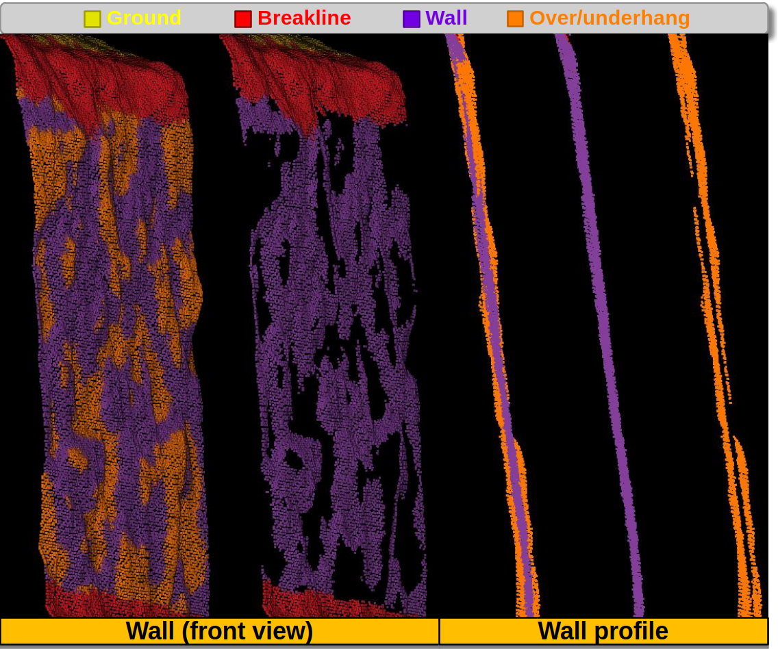
Visualization of the reclassified point cloud. Wall is purple, overhangs and underhangs are orange.

Taut string reclassifier

The TautStringReclassifier reclassifies points of a user-specified wall class as underhang when they lie deeper than a length threshold \(D\) below a locally fitted taut string surface envelope. The envelope is computed slice-by-slice on a per-cluster 2D profile (the cluster’s vertical axis vs. the horizontal direction orthogonal to its local plane normal) and bounded by a sliding vertical window so that a single long inward curvature of the wall does not saturate every point as an underhang. On each window the upper hull (Andrew’s monotone chain) plays the role of the taut string: any in-slice point whose vertical gap to the hull exceeds \(D\) is flagged as an underhang. The depth used to threshold and emit as the optional wall_depth feature is the max-aggregate across the \(w / s\) overlapping windows each interior point is visited by.

Wall clusters themselves come from a region-growing pass over the source_classes mask, seeded in deterministic input-cloud-index order and gated by a PCA plane-tolerance criterion (\(\lambda_3 \leq \tau^{2}\)) and a minimum-cluster-size guard. The cluster’s centred covariance gives the plane normal \(\pmb{n}\), which is sign-disambiguated against a horizontal direction \(\pmb{h}\) via the cross product with the gravity axis. To tell genuine inward concavities (underhangs) apart from outward protrusions (overhangs), the algorithm consults a hierarchy of signals derived from the cluster’s surrounding ground-class points: a majority side count, a “lower-ground median” tie-break, and a “lower-ground base” tie-break (see Mode A vs. mode B below). When ground_classes is not provided, the algorithm runs in a non-ambiguity-resolution fallback in which both the upper AND the lower convex hulls of each slice are computed and the larger of the two envelope gaps is the depth — any sufficiently deep deviation, inward or outward, is then labeled as underhang.

A TautStringReclassifier is intended for semantically- segmented 3D point clouds in which the wall class has already been predicted (e.g. by a deep-learning classifier upstream in the pipeline) and the operator wants to refine that prediction by carving out the genuinely concave or otherwise locally-deviating regions of each wall. The component is implemented as a thin Python wrapper over a multi-threaded C++ backend (mirroring DirectionalReclassifier) and exposes the same report / output-column controls. A TautStringReclassifier can be defined inside a pipeline using the JSON below:

{
    "class_transformer": "TautStringReclassifier",
    "on_predictions": true,
    "input_class_names": [
        "ground", "wall", "vegetation", "other", "break", "unlabeled"
    ],
    "source_classes": ["wall"],
    "underhang_class": "underhang",
    "output_class_names": [
        "ground", "wall", "underhang",
        "vegetation", "other", "break", "unlabeled"
    ],
    "depth_threshold": 0.2,
    "gravity_direction": [0, 0, 1],
    "bin_size": 0.05,
    "sliding_window_size": 5.0,
    "sliding_window_stride": 1.0,
    "plane_fit_trim": true,
    "plane_fit_trim_eps": 0,
    "initial_region_radius": 3.0,
    "region_growing_step": 1.0,
    "region_growing_plane_tolerance": 0.3,
    "ground_classes": ["ground"],
    "ground_search_radius": 0,
    "ground_min_count": 10,
    "ground_majority_ratio": 0.65,
    "ground_distance_deadband": 0,
    "ground_elevation_deadband": 0,
    "include_cluster_eigenmin": true,
    "cluster_eigenmin_name": "eigenmin",
    "include_wall_clusters": true,
    "wall_cluster_name": "wall_cluster",
    "include_depth_distance": true,
    "depth_distance_name": "wall_depth",
    "nthreads": -1,
    "report_path": null,
    "plot_path": null
}

The JSON above defines a TautStringReclassifier that operates on the "wall" class of the predictions, relabels concave points deeper than \(D = 0.2\) length-units as "underhang", and exports the per-point depth distance, the per-point wall cluster id, and the per-cluster plane-fit min eigenvalue as LAS extra dims for downstream auditing.

Algorithm and motivating math. The transform processes each wall cluster \(C\) independently. Let \(\pmb{\mu} = \frac{1}{|C|} \sum_{i \in C} \pmb{p}_{i}\) be the cluster centroid and let \(\pmb{\Sigma}\) be its centred covariance matrix. The plane normal \(\pmb{n}\) is the unit-norm eigenvector of \(\pmb{\Sigma}\) associated with the smallest eigenvalue \(\lambda_{3}\):

\[\pmb{\Sigma} = \frac{1}{|C|} \sum_{i \in C} (\pmb{p}_{i} - \pmb{\mu}) (\pmb{p}_{i} - \pmb{\mu})^{\intercal}, \qquad \pmb{\Sigma} \, \pmb{n} = \lambda_{3} \, \pmb{n}, \qquad \lambda_{3} = \min \mathrm{spec}(\pmb{\Sigma}).\]

When plane_fit_trim is true the PCA is refit after discarding points whose absolute signed distance to the first-pass plane exceeds \(\epsilon\) (auto-default \(\epsilon = D / 2\) if plane_fit_trim_eps is 0 or null).

When the user-supplied gravity direction \(\pmb{g}\) differs from \((0, 0, 1)\), the cluster is rotated into a frame in which the gravity axis is the world-\(z\) axis. Concretely the rotation matrix \(\pmb{B} \in \mathbb{R}^{3 \times 3}\) is any orthogonal matrix with \(\pmb{B} \, \pmb{g} = (0, 0, 1)^{\intercal}\); the centred cluster is then transformed as

\[\pmb{P}' = \pmb{B} \, (\pmb{P} - \pmb{\mu}).\]

In the rotated frame \(\pmb{e}_{3} = (0, 0, 1)\). The horizontal direction \(\pmb{h}\) and the slicing axis \(\pmb{s}\) are derived from the cluster’s plane normal \(\pmb{n}\) by projecting out the gravity component and then taking a horizontal cross product with \(\pmb{e}_{3}\):

\[\pmb{h} = \frac{(n_{x}, n_{y}, 0)} {\lVert (n_{x}, n_{y}, 0) \rVert}, \qquad \pmb{s} = \pmb{e}_{3} \times \pmb{h} = (-h_{y}, h_{x}, 0).\]

A hard-coded numerical gate \(\lVert (n_{x}, n_{y}, 0) \rVert < \epsilon_{h} = 10^{-3}\) declares the cluster as a near-horizontal “wall” (a floor / ceiling / flat roof mislabel) and skips it with a per-cluster warning and a dedicated near-horizontal signal in the report. \(\epsilon_h\) is not a user hyperparameter.

For each cluster point \(\pmb{p}_{i}\) the slicing-axis distance \(\tilde{d}_{i} = \pmb{p}_{i}^{\intercal} \pmb{s}\) is binned at the user-supplied resolution \(\Delta\),

\[\mathrm{SLICE\_ID}(\pmb{p}_{i}) = \left\lfloor \frac{\tilde{d}_{i}}{\Delta} \right\rfloor,\]

so that all cluster points within the same vertical strip of width \(\Delta\) along \(\pmb{s}\) belong to the same slice. Inside each slice the points are re-expressed in the 2D local frame

\[\tilde{x}_{i} = z_{i} \quad \text{(vertical coordinate in the cluster's local basis)}, \qquad \tilde{y}_{i} = \pmb{p}_{i}^{\intercal} \pmb{h} \quad \text{(horizontal protrusion)}.\]

The sliding window of size \(w\) and stride \(s\) traverses the cluster’s vertical range; on each window the upper convex hull of the in-window points (mode A) or both the upper AND lower convex hulls (mode B) are computed by Andrew’s monotone chain in \(\mathcal{O}(n \log n)\). For an in-window point \((\tilde{x}_{i}, \tilde{y}_{i})\), the upper-hull line segment \((x_{a}, y_{a}) \to (x_{b}, y_{b})\) with \(x_{a} \leq \tilde{x}_{i} \leq x_{b}\) defines the linearly interpolated envelope height

\[\hat{y}_{i}^{\,\text{up}} = y_{a} + (\tilde{x}_{i} - x_{a}) \frac{y_{b} - y_{a}}{x_{b} - x_{a}}.\]

In mode A (ground-based, conclusive cluster) the per-window depth distance is

\[d_{i} = \hat{y}_{i}^{\,\text{up}} - \tilde{y}_{i}.\]

In mode B (non-ambiguity-resolution or per-cluster fallback) the lower hull is interpolated analogously to obtain \(\hat{y}_{i}^{\,\text{lo}}\) and the per-window depth distance is

\[d_{i} = \max \bigl( \hat{y}_{i}^{\,\text{up}} - \tilde{y}_{i}, \; \tilde{y}_{i} - \hat{y}_{i}^{\,\text{lo}} \bigr).\]

Each interior point is visited by \(w / s\) overlapping windows (five with the defaults \(w = 5.0\), \(s = 1.0\)); the per-point depth recorded on the output column is the max-aggregate across those visits. The thresholding rule

\[d_{i} > D \;\;\Longrightarrow\;\; \text{point } i \text{ is reclassified as } \texttt{underhang}\]

then drives the class column rewrite at the end of the transform.

Arguments

– class_transformer

The factory discriminator string. Must be exactly "TautStringReclassifier" for this transformer. Resolved at pipeline load time by src/utils/ctransf_utils.py::CtransfUtils.extract_ctransf_class via case-insensitive name match against the registered class transformers.

– on_predictions

Whether to also reclassify the predictions if any (true) or not (false). Note that setting on_predictions to true will only work if predictions are available on the input point cloud.

– input_class_names

A list with the names of the input classes.

– source_classes

The names of the classes such that only points of these classes will be considered for the wall-clustering and reclassification computation. Points whose class is not in source_classes are not removed from the output cloud — they are simply ignored by the algorithm and preserved unchanged.

– underhang_class

The name of the underhang class. Must be a member of output_class_names AND must not appear in source_classes (relabeling a source class as itself is a no-op and is rejected at __init__).

– output_class_names

A list with the desired names for the output/transformed classes.

– depth_threshold

The depth \(D \in \mathbb{R}_{>0}\) at which a point’s vertical gap to the local upper convex hull is considered an underhang. Defaults to 0.2. Eager validation: must be a strictly positive finite scalar.

– gravity_direction

The unit-norm vector \(\pmb{g} \in \mathbb{R}^{3}\) pointing along the up axis (i.e. opposite the pull of gravity). Despite the name, this is the vertical axis oriented upward, not a downward acceleration vector; the naming is preserved for backwards compatibility with the framework’s other components. Defaults to [0, 0, 1]. Eager validation: exactly 3 components, Euclidean norm \(\geq 10^{-7}\). If supplied non-unit-norm, the vector is normalised internally and an INFO log message is emitted at setup.

– bin_size

The bin width \(\Delta \in \mathbb{R}_{>0}\) of the vertical slicing along \(\pmb{s}\). Defaults to 0.05. Eager validation: \(\Delta > 0\).

– sliding_window_size

The vertical size \(w \in \mathbb{R}_{>0}\) of the sliding window in length units of the input cloud. Defaults to 5.0. Eager validation: \(w > 0\) and \(w \geq s\) (the window must be at least as large as the stride, otherwise the sliding windows leave vertical gaps). Limiting the vertical span of the convex-hull computation prevents a slight inward curvature of a full wall (say \(d = 0.5\) depth at peak with \(D = 0.2\)) from saturating every point as an underhang.

– sliding_window_stride

The vertical step \(s \in \mathbb{R}_{>0}\) of the sliding window. Defaults to 1.0. Eager validation: \(s > 0\) and \(s \leq w\). With the defaults \(w = 5.0\) and \(s = 1.0\) each interior point is visited by 5 overlapping windows; the depth recorded on the output column is the max-aggregate across those visits. Smaller strides over-sample (more robust to local hull-anchoring artefacts at window boundaries) at the cost of redundant per-point hull-distance evaluations.

– plane_fit_trim

A bool. When true the PCA plane is refit after discarding points that deviate more than \(\epsilon\) from the first-pass plane, yielding a more accurate plane normal for clusters whose non-surface debris perturbs the PCA fit. Defaults to true.

– plane_fit_trim_eps

The trim threshold \(\epsilon \in \mathbb{R}_{\geq 0}\) for the optional plane refit. When given as 0 or null, the auto-default \(\epsilon = D / 2\) is used; otherwise the user-supplied value is used verbatim. Only relevant when plane_fit_trim is true. Defaults to 0.

– initial_region_radius

The initial spherical neighborhood radius \(r_{0} \in \mathbb{R}_{>0}\) used to seed the region-growing pass. Every wall point within \(r_{0}\) of the seed forms the initial region. Defaults to 3.0. Eager validation: \(r_{0} > 0\).

– region_growing_step

The radius \(r_{\Delta} \in \mathbb{R}_{>0}\) of each successive region-growing expansion after the initial region. Defaults to 1.0. Eager validation: \(r_{\Delta} > 0\).

– region_growing_plane_tolerance

The plane-tolerance threshold \(\tau \in \mathbb{R}_{\geq 0}\) for the region-growing PCA gate. Successive expansions are accepted only when the refit min eigenvalue \(\lambda_{3} \leq \tau^{2}\). The initial region is always accepted; on rejection the cluster falls back to the last accepted state (no backtracking, no iteration skip). Defaults to 0.3. When given as 0 or null the plane-tolerance gate is disabled.

– ground_classes

Optional list of class names representing the ground in input_class_names. Every entry must match a name in input_class_names exactly. Drives the algorithm’s mode:

• Mode A (ground-based ambiguity breaker, active when ``ground_classes`` is a non-empty list). For each wall cluster the algorithm queries the ground-class points surrounding the cluster centroid and uses them to disambiguate the sign of \(\pmb{h}\) via a three-tier signal hierarchy — primary majority side count (majority), secondary “lower-ground median” tie-break (lower-ground-median), tertiary “lower-ground base” tie-break (lower-ground-base). Only inward concavities (underhangs) are then reclassified; outward protrusions (overhangs) are preserved. An INFO log message at the start of every transform identifies the active mode and lists the ground class names.

• Mode B (non-ambiguity-resolution, active when ``ground_classes`` is ``null``, missing, or empty). The sign of \(\pmb{h}\) is left as PCA returned it. Both the upper AND the lower convex hulls of each slice are computed and the max-of-two-envelopes depth rule is applied; any sufficiently large deviation (inward OR outward) is labeled as underhang. Known caveat: surface points immediately adjacent to a large overhang or underhang may receive a false underhang label because the local convex hull is anchored by the deviation, lifting (resp. lowering) the envelope across a horizontal band bounded by sliding_window_size and the deviation’s projected width. The \(5\times\) sliding-window over-sampling reduces but does not eliminate the effect. Users who can supply ground_classes should do so — mode A removes the ambiguity at the root rather than mitigating it downstream.

See the dedicated Mode A vs. mode B contract sub-section below and the Per-cluster sign-disambiguation report sub-section for the full decision rule and the report contract.

– ground_search_radius

Radius \(R_{g} \in \mathbb{R}_{\geq 0}\) around each wall cluster centroid used to query ground points. Only applies in mode A. When given as 0 or null the auto-default \(R_{g} = 3 \, r_{0}\) is used (three times the initial_region_radius). When the first query returns fewer than ground_min_count points the radius is expanded once to \(2 R_{g}\) before declaring the cluster inconclusive. Defaults to 0.

– ground_min_count

Minimum count \(N_{g}^{\min} \in \mathbb{N}_{>0}\) of ground points required (after the optional radius expansion) for mode A to fire on a cluster. When fewer than \(N_{g}^{\min}\) ground points are found, the cluster falls back to mode-B treatment for that cluster only (a per-cluster warning is emitted into the report). Only applies in mode A. Defaults to 10.

– ground_majority_ratio

Side-count fraction \(\rho_{g}^{\min} \in (0.5, 1]\) at which the primary signal of the sign disambiguation commits to an outward direction. The orientation is taken as \(\mathrm{sign}(|G_{+}| - |G_{-}|)\) provided \(\max(|G_{+}|, |G_{-}|) / (|G_{+}| + |G_{-}|) \geq \rho_{g}^{\min}\). Otherwise the algorithm falls through to the lower-ground tie-breaks. Only applies in mode A. Defaults to 0.65.

– ground_distance_deadband

Signed-distance dead-band \(\delta_{g} \in \mathbb{R}_{\geq 0}\) (length units of the input cloud) applied when classifying each ground point as lying on the \(+\pmb{n}\) side, the \(-\pmb{n}\) side, or “on the plane”. Ground points with absolute signed distance below \(\delta_{g}\) are excluded from both side counts. When given as 0 or null the auto-default \(\delta_{g} = \Delta\) (one bin_size) is used. Only applies in mode A. Defaults to 0.

– ground_elevation_deadband

Vertical dead-band \(\tau_{z} \in \mathbb{R}_{\geq 0}\) (length units of the input cloud, measured along \(\pmb{g}\)) used by the secondary and tertiary “lower-ground” tie-breaks. When the median (secondary) or base-restricted minimum (tertiary) elevations of the two sides differ by less than \(\tau_{z}\) the tie-break is declared inconclusive and the algorithm proceeds to the next signal (or to the per-cluster mode-B fallback on the last tier). When given as 0 or null the auto-default \(\tau_{z} = r_{0}\) (one initial_region_radius) is used. Only applies in mode A. Defaults to 0.

– include_cluster_eigenmin

A bool. When true the smallest eigenvalue \(\lambda_3\) of the cluster’s last-accepted centered covariance is exposed as a per-point float32 LAS extra-dim. Defaults to false.

– cluster_eigenmin_name

The LAS extra-dim name for the per-point min eigenvalue. Must be a non-empty string. Only relevant when include_cluster_eigenmin is true. Defaults to "eigenmin".

– include_wall_clusters

A bool. When true the per-point wall cluster id is exposed as an int32 LAS extra-dim. Each accepted wall cluster is assigned a contiguous id in \([0, N - 1]\) in the seed-point-index order; non-wall points and points belonging to a skipped cluster (near-horizontal or rejected by the minimum-cluster guard) carry the sentinel value \(-1\). Defaults to false.

– wall_cluster_name

The LAS extra-dim name for the per-point wall cluster id. Must be a non-empty string. Only relevant when include_wall_clusters is true. Defaults to "wall_cluster".

– include_depth_distance

A bool. When true the per-point depth distance is exposed as a float32 LAS extra-dim. In mode A the depth is the signed gap below the upper envelope; in mode B (or in a per-cluster mode-A fallback) the depth is the max-of-two- envelopes gap. Wall points that were not touched by any window carry 0.0. Non-wall points all carry 0.0. Defaults to false.

– depth_distance_name

The LAS extra-dim name for the per-point depth distance. Must be a non-empty string. Only relevant when include_depth_distance is true. Defaults to "wall_depth".

– nthreads

The number of OpenMP threads for the parallel C++ execution. -1 means as many threads as available cores.

– report_path

Optional filesystem path. When provided, the TautStringReclassificationReport is persisted as a CSV at this path after each transform call. The CSV holds the per-cluster sign-disambiguation trace described in Per-cluster sign-disambiguation report below. When null, missing, or empty, the report is emitted only to the log through the ClassTransformer.report machinery.

– plot_path

Accepted in the JSON for schema compatibility with the rest of the class-transformer family but not used in this iteration of the TautStringReclassifier — unlike DirectionalReclassifier / DirectionalReclassificationPlot, no companion plot class is generated. A future iteration may add a TautStringReclassificationPlot; until then, do not rely on plot output.

Output

The output is a point cloud with the same coordinates and feature space as the input but with classifications (or predictions) updated according to the taut-string reclassification rules described above. Non-source-class points are preserved. When several sliding windows visit the same point, the largest per-window depth wins (the max-aggregate is computed per-cluster in the C++ backend; each wall point belongs to exactly one cluster after region growing, so each output column entry has a unique writer thread and no atomics are required). The transform optionally emits up to three LAS extra-dim columns described below.

– <cluster_eigenmin_name> (float32, default name

"eigenmin") The smallest eigenvalue \(\lambda_3\) of the wall cluster’s last-accepted centered covariance matrix. A measure of how planar the cluster is — small values mean a well-fit plane, large values mean the cluster grew across non-planar geometry. The sentinel value on points that are not in any accepted wall cluster (including non-wall points, near-horizontal-skipped cluster members, and minimum-cluster-guard rejects) is 0.0. Note that 0.0 is also numerically valid for a perfectly planar cluster; disambiguate via the cluster id column if needed.

– <wall_cluster_name> (int32, default name

"wall_cluster") The per-point wall cluster id. Accepted wall clusters are assigned a contiguous id in \([0, N - 1]\) in the seed-point-index order. The sentinel value on points that do not participate in any accepted wall cluster is \(-1\). inconclusive and pure mode-B clusters DO participate in cluster-id assignment (both ran through the full pipeline, just under the dual-hull treatment); near-horizontal-skipped clusters AND clusters rejected by the minimum-cluster guard DO NOT participate.

– <depth_distance_name> (float32, default name

"wall_depth") The max-aggregate per-point depth distance across all windows that visited the point. In mode A this is the canonical underhang depth \(d_{i} = \hat{y}_{i}^{\,\text{up}} - \tilde{y}_{i}\); in mode B (or in a per-cluster mode-A fallback) it is the max-of-two-envelopes depth \(d_{i} = \max(\hat{y}_{i}^{\,\text{up}} - \tilde{y}_{i}, \tilde{y}_{i} - \hat{y}_{i}^{\,\text{lo}})\). The sentinel value on points that were not visited by any window (including non-wall points and accepted-cluster wall points untouched by the sliding window) is 0.0.

Mode A vs. mode B contract

The presence of the ground_classes hyperparameter selects between two complementary code paths inside the transform, hereafter called mode A and mode B:

• Mode A is active when ground_classes is provided as a non-empty list of class names. The algorithm queries the points of those classes around each wall cluster centroid and uses them to break the underhang-vs-overhang sign ambiguity via a three-tier signal hierarchy:

  1. Primary signal — majority side wins. The signed distance \(d_{j} = (\pmb{p}_{j} - \pmb{\mu})^{\intercal} \pmb{n}\) is computed for every ground point \(\pmb{p}_{j}\) in the candidate set; the two side counts \(|G_{+}|, |G_{-}|\) are formed after the dead-band filter \(|d_{j}| > \delta_{g}\). When the dominant side holds a fraction \(\geq \rho_{g}^{\min}\) of the qualified ground points, its sign becomes outward and the signal is recorded as majority.

  2. Secondary signal — lower-ground median tie-break. When the side counts are too close, the median elevation of the ground points on each side (in the original gravity frame) is compared; the side whose median is lower by more than \(\tau_{z}\) is outward and the signal is recorded as lower-ground-median.

  3. Tertiary signal — base-level lower-ground tie-break. When the medians are also within \(\tau_{z}\) of each other, ground points within \(r_{0}\) upward of the cluster base elevation are restricted; the side whose base-restricted minimum elevation is lower by more than \(\tau_{z} / 2\) is outward and the signal is recorded as lower-ground-base.

  Only inward concavities (underhangs) are reclassified in mode A. Outward protrusions (overhangs) are preserved unchanged. A per-cluster warning is emitted whenever a cluster’s signal hierarchy is exhausted without a conclusive result (signal inconclusive); the cluster then falls back to mode-B treatment for that cluster only (see below).

• Mode B is active when ground_classes is null, missing, or an empty list. The sign of \(\pmb{h}\) is left as PCA returned it. For each slice the algorithm computes BOTH the upper AND the lower convex hulls and assigns to each point the maximum of its two depth distances; any point whose max depth exceeds \(D\) is reclassified as underhang regardless of direction. Mode B is therefore strictly less informative than mode A — it catches both inward concavities and outward protrusions — but requires no ground-class context. The known caveat is a false-positive band near large deviations (see the ground_classes argument).

• Per-cluster mode-A inconclusive fallback. When mode A’s signal hierarchy exhausts without a conclusive result on a single cluster, that cluster falls back to the mode-B dual-hull treatment while the rest of the clusters in the same transform continue under mode A. The fallback is logged in the per-cluster report under the signal value inconclusive.

The Arguments section above spells out the mode-A vs mode-B contract of ground_classes and links to the per-cluster sign- disambiguation report format documented in the next sub-section.

Per-cluster sign-disambiguation report

When report_path is provided, the transform persists a CSV file that holds one row per wall cluster (including skipped clusters). The CSV is generated by TautStringReclassificationReport and written by its to_file(path, out_prefix=None) method. The columns are, in order:

• seed_point_idx

  The input-cloud index of the cluster’s seed point (the smallest member point index). This is the canonical row sort key.

• cluster_idx

  The densified cluster id assigned to the cluster (the cluster’s rank in the seed-point-index ordering). The value is \(-1\) for skipped clusters (near-horizontal and minimum-cluster-guard rejects) since they do not participate in cluster-id assignment.

• centroid_x, centroid_y, centroid_z

  The cluster centroid \(\pmb{\mu} \in \mathbb{R}^{3}\) (world coordinates, before the gravity-based change of basis).

• point_count

  The number of points in the cluster.

• mode

  The mode under which the cluster was processed: A for a conclusive mode-A cluster, B for a pure mode-B cluster (the transform itself runs in mode B) or a per-cluster fallback cluster from mode A, and skipped for clusters that were not processed because of the near-horizontal gate or the minimum-cluster guard.

• signal

  The signal that decided the orientation: majority, lower-ground-median, lower-ground-base, inconclusive, near-horizontal, or pure-mode-B.

• g_plus_count, g_minus_count

  The side counts \(|G_{+}|\) and \(|G_{-}|\) at the moment of the primary-signal decision. Zero for mode-B and skipped clusters.

• z_plus_median, z_minus_median

  The median elevations of the two sides used by the secondary signal (lower-ground-median). NaN for clusters that short-circuited at the primary signal.

• z_plus_min_base, z_minus_min_base

  The base-restricted minimum elevations used by the tertiary signal (lower-ground-base). NaN for clusters that short-circuited earlier.

• n_horizontal_norm

  The recorded \(\lVert (n_{x}, n_{y}, 0) \rVert\) value for clusters that triggered the near-horizontal skip. NaN for every other cluster.

The per-cluster trace is emitted via the report only; it does not pollute the main INFO log channel. The transform itself emits exactly two main-channel INFO log messages: a start-of-transform message identifying the active mode (mode A with the ground class names, or mode B) and an end-of-transform message summarising how many clusters resolved via each signal — N_A_majority, N_A_lower_median, N_A_lower_base, N_A_inconclusive, N_B_pure_mode_B, N_skipped_near_horizontal, N_skipped_too_small — plus the total wall-cluster count and the count of reclassified points. Per-cluster WARNINGs for inconclusive and near-horizontal clusters and DEBUG load notices follow the existing per-level logging conventions used by DirectionalReclassifier.

Feature transformers

Minmax normalizer

The MinmaxNormalizer maps the specified features so they are inside the \([a, b]\) interval. It can be configured to clip values outside the interval or not. If so, values below \(a\) will be replaced by \(a\) while values above \(b\) will be replaced by \(b\). A MinmaxNormalizer can be defined inside a pipeline using the JSON below:

{
    "feature_transformer": "MinmaxNormalizer",
    "fnames": ["AUTO"],
    "target_range": [0, 1],
    "clip": true,
    "report_path": "minmax_normalization.log"
}

The JSON above defines a MinmaxNormalizer that will map the features to be inside the \([0, 1]\) interval. If this transformer is later applied to different data, it will make sure that there is not value less than zero or greater than one. On top of that, a report about the normalization will be written to the minmax_normalization.log text file.

Arguments

– fnames

The names of the features to be normalized. If "AUTO", the features considered by the last component that operated over the features will be used.

– target_range

The interval to normalize the features.

– clip

When a minmax normalizer has been fit to a dataset, it will find the min and max values to compute the normalization. It can be that the normalizer is then applied to other dataset with different min and max. Under those circumstances, values below \(a\) or above \(b\) might appear. When clip is set to true, this values will be replaced by either \(a\) or \(b\) so the normalizer never yields values outside the \([a, b]\) interval.

– minmax

An optional list of pairs (e.g., list of lists, where each sublist has exactly two elements). When given, each i-th element is a pair where the first component gives the min for the i-th feature and the second one gives the max.

– frenames

An optional list of names. When given, the normalized features will use these names instead of the original ones given by fnames.

– report_path

When given, a text report will be exported to the file pointed by the path.

– update_and_preserve

When true, the features that were not transformed by minmax normalization will be kept in the point cloud with the normalized features. When false, the values of non-transformed features might be missing.

Output

A transformed point cloud is generated such that its features are normalized to a [0, 1] interval. The min, the max, and the range are exported through the logging system (see below for an example corresponding to the minmax normalization of some geometric features).

FEATURE	MIN	MAX	RANGE
linearity_r0.05	0.00028	1.00000	0.99972
planarity_r0.05	0.00000	0.97660	0.97660
surface_variation_r0.05	0.00000	0.32316	0.32316
eigenentropy_r0.05	0.00006	0.01507	0.01501
omnivariance_r0.05	0.00000	0.00060	0.00060
verticality_r0.05	0.00000	1.00000	1.00000
anisotropy_r0.05	0.06250	1.00000	0.93750
linearity_r0.1	0.00070	1.00000	0.99930
planarity_r0.1	0.00000	0.95717	0.95717
surface_variation_r0.1	0.00000	0.32569	0.32569
eigenentropy_r0.1	0.00028	0.04501	0.04473
omnivariance_r0.1	0.00000	0.00241	0.00241
verticality_r0.1	0.00000	1.00000	1.00000
anisotropy_r0.1	0.05643	1.00000	0.94357

Standardizer

The Stantardizer maps the specified features so they are transformed to have mean zero \(\mu = 0\) and standard deviation one \(\sigma = 1\). Alternatively, it is possible to only center (mean zero) or scale (standard deviation one) the data. A Standardizer can be defined inside a pipeline using the JSON below:

{
    "feature_transformer": "Standardizer",
    "fnames": ["AUTO"],
    "center": true,
    "scale": true,
    "report_path": "standardization.log"
}

The JSON above defines a Standardizer that centers and scales the data. Besides, it will export a text report with the feature-wise means and variances to the standardization.log file.

Arguments

– fnames

The names of the features to be standardized. If "AUTO", the features considered by the last component that operated over the features will be used.

– center

Whether to subtract the mean (true) or not (false).

– scale

Whether to divide by the standard deviation (true) or not (false).

– frenames

An optional list of names. When given, the standardized features will use these names instead of the original ones given by fnames.

– report_path

When given, a text report will be exported to the file pointed by the path.

– update_and_preserve

When true, the features that were not transformed through normalization (i.e., standardization) will be kept in the point cloud with the normalized features. When false, the values of non-transformed features might be missing.

Output

A transformed point cloud is generated such that its features are standardized. The mean and standard deviation are exported through the logging system (see below for an example corresponding to the standardization of some geometric features).

FEATURE	MEAN	STDEV.
linearity_r0.05	0.47259	0.24131
planarity_r0.05	0.32929	0.22213
surface_variation_r0.05	0.10697	0.06362
eigenentropy_r0.05	0.00781	0.00184
omnivariance_r0.05	0.00025	0.00010
verticality_r0.05	0.55554	0.30274
anisotropy_r0.05	0.80188	0.14316
linearity_r0.1	0.49389	0.24075
planarity_r0.1	0.29196	0.21008
surface_variation_r0.1	0.11583	0.06376
eigenentropy_r0.1	0.02512	0.00533
omnivariance_r0.1	0.00100	0.00035
verticality_r0.1	0.57260	0.30121
anisotropy_r0.1	0.78585	0.14570

Variance selector

The variance selection is a simple strategy that consists of discarding all those features which variance lies below a given threshold. While simple, the VarianceSelector has a great strength and that is it can be computed without known classes because it is based only on the variance. A VarianceSelector can be defined inside a pipeline using the JSON below:

{
    "feature_transformer": "VarianceSelector",
    "fnames": ["AUTO"],
    "variance_threshold": 0.01,
    "report_path": "variance_selection.log"
}

The JSON above defines a VarianceSelector that removes all features which variance is below \(10^{-2}\). After that, it will export a text report describing the process to the variance_selection.log file.

Arguments

– fnames

The names of the features to be transformed. If "AUTO", the features considered by the last component that operated over the features will be used.

– variance_threshold

Features which variance is below this threshold will be discarded.

– report_path

When given, a text report will be exported to the file pointed by the path.

Output

A transformed point cloud is generated considering only the features that passed the variance threshold. On top of that, the feature-wise variances are exported through the logging system. The selected features are also explicitly listed (see below for an example corresponding to a variance selection on some geometric features).

FEATURE	VARIANCE
omnivariance_r0.05	0.000
omnivariance_r0.1	0.000
eigenentropy_r0.05	0.000
eigenentropy_r0.1	0.000
surface_variation_r0.05	0.004
surface_variation_r0.1	0.005
anisotropy_r0.05	0.020
anisotropy_r0.1	0.022
linearity_r0.1	0.051
linearity_r0.05	0.056
planarity_r0.1	0.066
planarity_r0.05	0.075
verticality_r0.05	0.092
verticality_r0.1	0.097

SELECTED FEATURES
linearity_r0.05
planarity_r0.05
verticality_r0.05
anisotropy_r0.05
linearity_r0.1
planarity_r0.1
verticality_r0.1
anisotropy_r0.1

K-Best selector

The KBestSelector computes the feature-wise ANOVA F-values and use them to sort the features. Then, only the \(K\) best features, i.e., those with highest F-values, will be preserved. A KBestSelector can be defined inside a pipeline using the JSON below:

{
    "feature_transformer": "KBestSelector",
    "fnames": ["AUTO"],
    "type": "classification",
    "k": 2,
    "report_path": "kbest_selection.log"
}

The JSON above defines a KBestSelector that computes the ANOVA F-Values assuming a classification task. Then, it discards all features but the two with the highest values. Finally, it writes a text report with the feature-wise F-Values and the associated p-value for each test to the file kbest_selection.log

Arguments

– fnames

The names of the features to be transformed. If "AUTO", the features considered by the last component that operated over the features will be used.

– type

Specify which type of task is going to be computed. Either, "regression" or "classification". The F-Values computation will be carried out to be adequate for one of those tasks. For regression tasks the target variable is expected to be numerical, while for classification tasks it is expected to be categorical.

– k

How many top-features must be preserved.

– report_path

When given, a text report will be exported to the file pointed by the path.

Output

A transformed point cloud is generated considering only the K-best features according to the F-values. Moreover, the feature-wise F-Values and their associated p-value are exported through the logging system. The selected features are also explicitly listed (see below for an example corresponding to a K-best selection on some geometric features).

FEATURE	F-VALUE	P-VALUE
eigenentropy_r0.1	811.946	0.000
omnivariance_r0.05	1050.085	0.000
linearity_r0.05	2290.284	0.000
planarity_r0.1	4795.994	0.000
linearity_r0.1	16100.821	0.000
eigenentropy_r0.05	16307.772	0.000
anisotropy_r0.05	17643.102	0.000
surface_variation_r0.05	18972.138	0.000
planarity_r0.05	19226.943	0.000
omnivariance_r0.1	20649.736	0.000
verticality_r0.05	90577.769	0.000
verticality_r0.1	106840.172	0.000
anisotropy_r0.1	116002.960	0.000
surface_variation_r0.1	122409.281	0.000

SELECTED FEATURES
surface_variation_r0.1
anisotropy_r0.1

Percentile selector

The PercentileSelector computes the ANOVA F-Values and use them to sort the features. Then, only a given percentage of the features are preserved. More concretely, the given percentage of the features with the highest F-Values will be preserved. A PercentileSelector can be defined inside a pipeline using the JSON below:

{
    "feature_transformer": "PercentileSelector",
    "fnames": ["AUTO"],
    "type": "classification",
    "percentile": 20,
    "report_path": "percentile_selection.log"
}

The JSON above defines a PercentileSelector that computes the ANOVA F-Values assuming a classification task. Then, it preserves the \(20\%\) of the features with the highest F-Values. Finally, it writes a text report with the feature-wise F-Values and the associated p-value for each test to the file percentile_selection.log.

Arguments

– fnames

The names of the features to be transformed. If "AUTO", the features considered by the last component that operated over the features will be used.

– type

Specify which type of task is going to be computed. Either, "regression" or "classification". The F-Values computation will be carried out to be adequate for one of those tasks. For regression tasks the target variable is expected to be numerical, while for classification tasks it is expected to be categorical.

– percentile

An integer from \(0\) to \(100\) that specifies the percentage of top-features to preserve.

– report_path

When given, a text report will be exported to the file pointed by the path.

Output

A transformed point cloud is generated considering only the requested percentage of best features according to the F-values. Moreover, the feature-wise F-Values and their p-value are exported through the logging system. The selected features are also explicitly listed (see below for an example corresponding to a percentile selection on some geometric features).

FEATURE	F-VALUE	P-VALUE
eigenentropy_r0.1	811.946	0.000
omnivariance_r0.05	1050.085	0.000
linearity_r0.05	2290.284	0.000
planarity_r0.1	4795.994	0.000
linearity_r0.1	16100.821	0.000
eigenentropy_r0.05	16307.772	0.000
anisotropy_r0.05	17643.102	0.000
surface_variation_r0.05	18972.138	0.000
planarity_r0.05	19226.943	0.000
omnivariance_r0.1	20649.736	0.000
verticality_r0.05	90577.769	0.000
verticality_r0.1	106840.172	0.000
anisotropy_r0.1	116002.960	0.000
surface_variation_r0.1	122409.281	0.000

SELECTED FEATURES
surface_variation_r0.1
verticality_r0.1
anisotropy_r0.1

Explicit selector

The ExplicitSelector preserves or discards the requested features, thus effectively updating the point cloud in the pipeline’s state (see SimplePipelineState). This feature transformation can be especially useful to release memory resources by discarding features that are not going to be used by other components later on. A ExplicitSelector can be defined inside a pipeline using the JSON below:

{
    "feature_transformer": "ExplicitSelector",
    "fnames": [
        "floor_distance_r50_0_sep0_35"
        "scan_angle_rank_mean_r5_0",
        "verticality_r25_0"
    ],
    "preserve": true
}

The JSON above defines a ExplicitSelector that preserves the floor distance, mean scan angle, and verticality features. In doing so, all the other features are discarded. After calling this selector, only the preserved features will be available through the pipeline’s state.

Arguments

– fnames

The names of the features to be either preserved or discarded.

– preserve

The boolean flag that governs whether the given features must be preserved (true) or discarded (false).

Output

A transformed point cloud is generated considering only the preserved features.

PCA transformer

The PCATransformer can be used to compute a dimensionality reduction of the feature space. Let \(\pmb{F} \in \mathbb{R}^{m \times n_f}\) be a matrix of features such that each row \(\pmb{f}_{i} \in \mathbb{R}^{n_f}\) represents the \(n_f\) features for a given point \(i\). After applying the PCA transformer a new matrix of features will be obtained \(\pmb{Y} \in \mathbb{R}^{m \times n_y}\) such that \(n_y \leq n_f\). This dimensionality reduction can help reducing the number of input features for a machine learning model, and consequently reducing the execution time.

To understand this transformation, simply note the singular value decomposition of \(\pmb{F} = \pmb{U} \pmb{\Sigma} \pmb{V}^\intercal\). The singular vectors in \(\pmb{V}^\intercal\) can be ordered in descendant order from higher to lower singular value, where singular values are given by the diagonal of \(\pmb{\Sigma}\). Alternatively, the basis matrix defined by the singular vectors can be approximated with the eigenvectors of the centered covariance matrix. From now on, no matter how it was computed, we will call this basis matrix \(\pmb{B}\). We also assume that we always have enough linearly independent features for the analysis to be feasible.

When all the basis vectors are considered, it will be that \(\pmb{B} \in \mathbb{R}^{n_f \times n_f}\), i.e., \(n_y=n_f\). In this case we are expressing potentially correlated features in a new basis where each feature aims to be orthogonal w.r.t. the others (principal components). When \(\pmb{B} \in \mathbb{R}^{n_f \times n_y}\) for \(n_y<n_f\), and the basis contains the singular vectors corresponding to the higher singular values , we are reducing the dimensionality using a subset of the principal components. This dimensionality reduction transformation will preserve as much variance as possible in the data while using less orthogonal features.

A PCATransformer can be defined inside a pipeline using the JSON below:

{
    "feature_transformer": "PCATransformer",
    "fnames": ["AUTO"],
    "out_dim": 0.99,
    "whiten": false,
    "random_seed": null,
    "report_path": "pca_projection.log",
    "plot_path": "pca_projection.svg",
    "update_and_preserve": false
}

The JSON above defines a PCATransformer that considers as many principal components as necessary to explain the \(99\%\) of the variance. On top of that, it will export a text report with the aggregated contribution to the explained variance of the considered principal components (ordered from most significant to less significant) to a file named pca_projection.log. Finally, it will also export a plot representing the explained variance ratio as a function of the output dimensionality to a file named pca_projection.svg.

Arguments

– fnames

The names of the features to be transformed. If "AUTO", the features considered by the last component that operated over the features will be used.

– out_dim

The ratio of preserved features governing the output dimensionality. It is a value in \((0, 1]\) where 1 implies \(n_y=n_f\) and less than one governs how small is \(n_y\) with respect to \(n_f\).

– whiten

When true, the singular vectors will be scaled by the square root of the number of points and divided by the corresponding singular value. Consequently, the output will consists of features with unit variance. When false, nothing will be done.

– random_seed

Can be used to specify a seed (as an integer) for reproducibility purposes when using randomized solvers for the computations.

– report_path

When given, a text report will be exported to the file pointed by the path.

– plot_path

When given, a plot representing the explained variance ratio as a function of the number of considered principal components will be exported to the file pointed by the path.

– update_and_preserve

When true, the features transformed through PCA will be discarded, but those that were not considered will be kept in the point cloud together with the PCA-based features. When false (by default), the point cloud will only contain the PCA-based features.

Output

A transformed point cloud is generated with the new features obtained by the PCATransformer. Moreover, the explained variances will be exported through the logging system.

FEATURE	EXPLAINED VAR. (%)
PCA_8	2.9685
PCA_7	3.9065
PCA_6	5.5666
PCA_5	6.9705
PCA_4	9.0035
PCA_3	12.0645
PCA_2	22.4750
PCA_1	36.2546

Furthermore, if requested a plot will be exported to a file. This plot describes the explained variance ratio as a function of the number of output features (output dimensionality). An example can be see below where the PCATransformer was used to reduce 14 features into 8 features that explain at least a \(99\%\) of the variance.

The relationship between the PCA-derived features and the aggregated explained variance ratio.

Finally, the image below represents how three different features were reduced to a single one using PCA. The output point cloud can be exported using a Writer component (see Writer documentation).

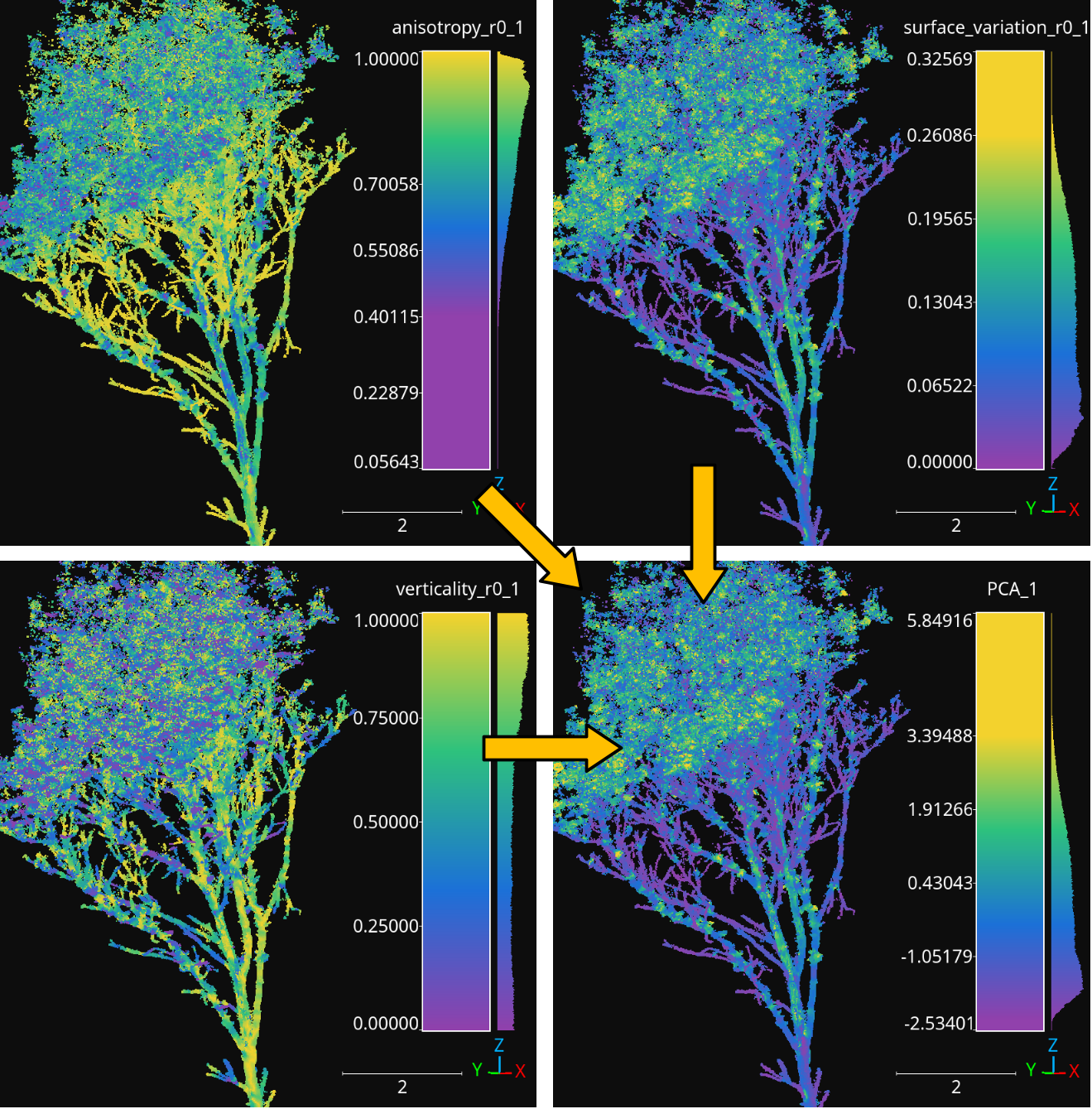
The anisotropy, surface variation, and verticality computed for spherical neighborhoods with \(10\,\mathrm{cm}\) radius reduced to a single feature through PCA.

Point transformers

Some point transformers like ReceptiveField or DataAugmentor and their derived classes (e.g., ReceptiveFieldFPS, ReceptiveFieldGS, ReceptiveFieldHierarchicalFPS, SimpleDataAugmentor )are used in the context of deep learning models. Thus, they are not available as independent components for pipelines. Other point transformers, typically those that extend PointTransformer can be used as components in pipelines and are detailed here.

Point cloud sampler

The PointCloudSampler generates a new point cloud by sampling from the current one (i.e., the point cloud in the pipeline’s state, see documentation on pipelines). A PointCloudSampler can be defined inside a pipeline using the JSON below:

{
    "point_transformer": "PointCloudSampler",
    "neighborhood_sampling": {
        "support_conditions": [
            {
                "value_name": "HighCA_rel",
                "condition_type": "greater_than_or_equal_to",
                "value_target": 0.667,
                "action": "preserve"
            }
        ],
        "support_min_distance": 1.25,
        "support_strategy": "fps",
        "support_strategy_num_points": 100000,
        "support_strategy_fast": true,
        "support_chunk_size": 50000,
        "center_on_pcloud": false,
        "neighborhood": {
            "type": "sphere",
            "radius": 2.5,
            "separation_factor": 0
        },
        "neighborhoods_per_iter": 10000,
        "nthreads": -1
    }
}

The JSON above defines a PointCloudSampler that will generate a point cloud considering spherical neighborhoods with radius \(2.5\,\mathrm{m}\) centered on those points in the current point cloud with a relative frequency of high class ambiguity neighbors greater than or equal to \(0.667\). A point is said to have a high class ambiguity if it is greater than or equal to \(0.667\). When sampling, all the center points that are close to each other in less than \(1.25\,\mathrm{m}\).

Arguments

– fnames

The names of the features that must be included in the sampled point cloud. If null, then all the available features will be included.

– neighborhood_sampling

When null, no neighborhood sampling will be applied. If given, it must be a key-word specification of the desired neighborhood sampling strategy, as described below:

– support_conditions

A list with the conditions that must be satisfied by any center point whose neighborhood could be included in the generated point cloud (provided it satisfies the other criteria). The specification for each conditions is similar to the one described in the conditions for advanced input documentation.

– support_min_distance

When more there are many center points that are close to each other in less than this distance, only one will be considered.

– support_strategy

If the support points are not calculated with a null separation factor, then the support strategy will be used to select the initial candidates. See the receptive fields documentation for further details because the specification works in the same way.

– support_strategy_num_points

If the support points are not calculated with a null separation factor, and the "fps" support strategy is used, then this number of points will govern the number of initially selected candidates. See the receptive fields documentation for further details because the specification works in the same way.

– support_strategy_fast

If the support points are not calculated with a null separation factor, fast heuristics can be applied to speedup the computations. See FPS receptive field documentation for further details.

– support_chunk_size

When given and distinct than zero, it will define the chunk size. The chunk size will be used to group certain tasks into chunks with a max size to prevent memory exhaustion.

– center_on_pcloud

When true the neighborhoods will be centered on a point from the input point cloud. Typically by finding the nearest neighbor of a support point in the input point cloud. In general, it is recommended to set it to false for most use cases of the PointCloudSampler.

– neighborhoods_per_iter

When doing multiple iterations to compute the neighborhoods, the overlapping might yield many repeated points. However, there is no need to store repeated elements in memory (which can be prohibitive). When the number of neighborhoods per iter is set to be greater than zero, only this number of neighborhoods will be computed at once, thus controlling the required memory.

– nthreads

The number of threads involved in parallel computations, if any.

– neighborhood

The definition of the neighborhood. See the FPS neighborhood specification for further details because it follows the same format.

– type

Supported neighborhood types are: "sphere", "cylinder", "rectangular3d", and "rectangular2d".

– radius

A decimal number goverening the size of the neighborhood.

– separation_factor

A decimal number governing the separation between neighborhoods. It it recommended to set it to zero so the custom support extraction strategy of the PointCloudSampler is used.

Output

A point cloud is generated by sampling spherical neighborhoods from high class ambiguity regions in the original point cloud. The class ambiguity has been measured for a KPConv-like neural network model. The point cloud is taken from the Architectural Cultural Heritage (ArCH) dataset .

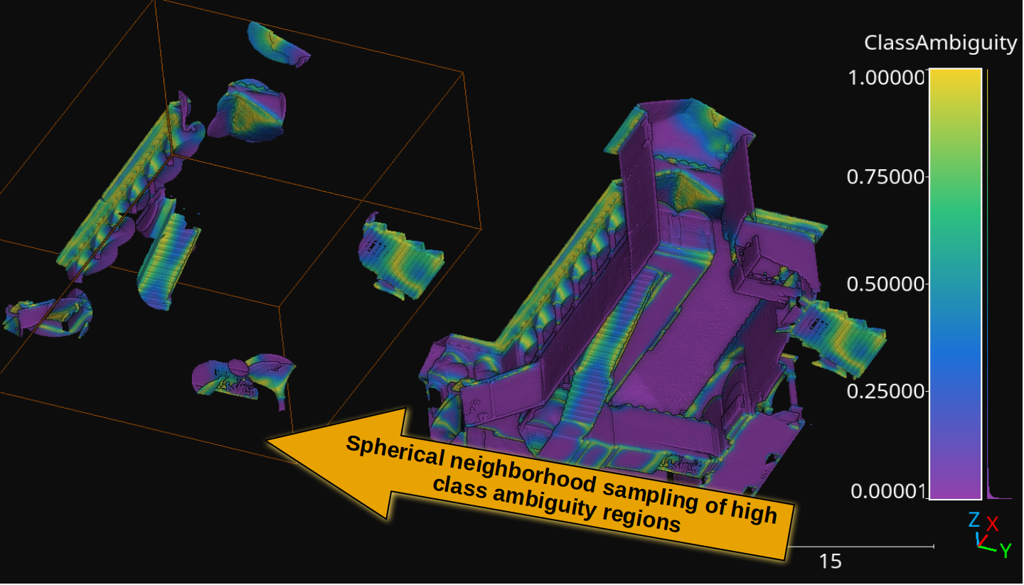
The spherical neighborhoods sampled from high class ambiguity regions (those inside the orange bounding box). The points are colored by class ambiguity.

Simple structure smoother++

The SimpleStructureSmootherPP generates a new point cloud by smoothing the coordinates of each point considering its local neighborhood. A SimpleStructureSmootherPP can be defined inside a pipeline using the JSON below:

{
  "point_transformer": "SimpleStructureSmootherPP",
  "neighborhood": {
    "type": "sphere",
    "radius": 20,
    "k": 1024
  },
  "strategy": {
    "type": "idw",
    "parameter": 2,
    "min_distance": 4
  },
  "correction": {
    "K": 0,
    "sigma": 3.14159265358979323846264338327950288419716939937510
  },
  "nthreads": -1
}

The JSON above defines a SimpleStructureSmoother applied on spherical neighborhoods with \(20\;\mathrm{mm}\) radius using inverse distance weighting with \(p=2\) and \(\epsilon=4\). It does not use Fibonacci orthodromic correction at all.

Arguments

– neighborhood

The definition of the neighborhood.

– type

The type of neighborhood. It can be either "knn" (3D k-nearest neighbors), "knn2d" (2D k-nearest neighbors considering the \((x, y)\) coordinates only), "sphere" (spherical neighborhood), and "cylinder" (cylindrical neighborhood).

– radius

The radius for the sphere or the disk of the cylinder.

– k

The number of k-nearest neighbors.

– strategy

The specification of the smoothing strategy.

– type

The smoothing strategy. It can be either "mean", "idw" (Inverse Distance Weighting), or "rbf" (Radial Basis Function).

– parameter

The \(p \in \mathbb{R}\) parameter for the IDW exponent or the Gaussian RBF bandwith.

– min_distance

The \(\epsilon \in \mathbb{R}\) parameter governing the min distance for IDW smoothing. Distances smaller than this will be replaced.

– correction

The configuration of the Fibonacci orthodromic correction.

– K

The number of pionts in the spherical Fibonacci support. The greater the better but it will lead to higher execution times (i.e., it increases the computational cost).

– sigma

The hard cut threshold for the Fibonacci orthodromic correction between a point in a centered neighborhood \(\pmb{x}_{j*} \in \mathbb{R}^{3}\) and a point from the Fibonacci support \(\pmb{q}_{k*} \in \mathbb{R}^{3}\).

\[\omega(\pmb{x}_{j*}, \pmb{q}_{k*}) = \max \left\{ 0, \sigma - \arccos\left(\dfrac{ \langle\pmb{x}_{j*}, \pmb{q}_{k*}\rangle }{ \lVert\pmb{x}_{j*}\rVert } \right) \right\}\]

– nthreads

The number of threads to be used for parallel computations (-1 means as many threads as available cores).

Output Smoother versions of a point cloud using the JSON above with different parameters. The input data comes from the Head and Neck Organ-at-Risk CT Segmentation Dataset (HaN-Seg) dataset.

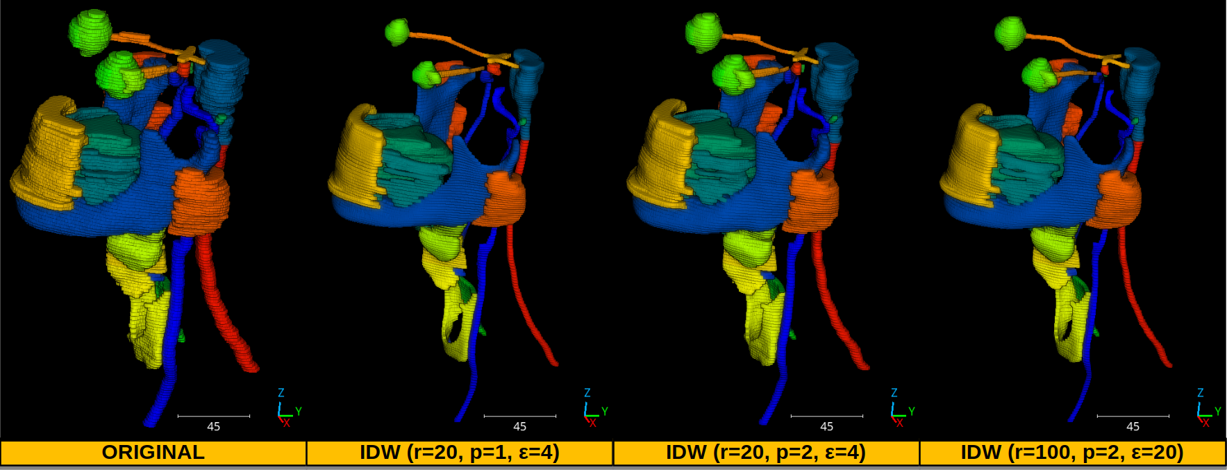
The smoothed versions of a medical 3D point cloud representing the head and neck regions. Each color represents a distinct organ.