Clustering

Clustering consists of receiving an input point cloud and finding points that can be grouped together into clusters. The clusters are typically represented with integer values \(c \in \mathbb{Z}_{\geq -1}\), where the value \(-1\) is used to represent no cluster or noise cluster. Clustering computations are carried out through Clusterer components. They can be included in pipelines. Besides, it is possible to define a post-processing pipeline that will be computed immediately after the clustering.

Clusterers

DBScan clusterer

The DBScanClusterer can be used to compute Density-Based Spatial Clustering of Applications with Noise (DBSCAN) in the point cloud. The DBSCAN algorithm considers a minimum number of points and a radius to define the neighborhood for spatial queries. It finds kernel points, those in whose neighborhood there are at least the minimum number of points. Then, it considers any accessible point to be in the cluster. The accessible points that are not kernel points are included in the cluster because they are close enough to the kernel points. However, these points are not considered to include new points as only kernel points can be used to determine whether a point is accessible or not. The JSON below shows how to define a DBScan clustering component:

{
    "clustering": "fpsdecorated",
    "fps_decorator": {
        "num_points": "m/10",
        "fast": true,
        "num_encoding_neighbors": 1,
        "num_decoding_neighbors": 1,
        "release_encoding_neighborhoods": false,
        "threads": 16,
        "representation_report_path": null
    },
    "decorated_clusterer": {
        "clustering": "dbscan",
        "cluster_name": "cluster_wood",
        "precluster_name": "Prediction",
        "precluster_domain": [1],
        "min_points": 200,
        "radius": 3.0,
        "post_clustering": [
            {
                "post-processor": "ClusterEnveloper",
                "envelopes": [
                    {
                        "type": "AlignedBoundingBox",
                        "compute_volume": true,
                        "output_path": "*/aabbs.csv",
                        "separator": ","
                    },
                    {
                        "type": "BoundingBox",
                        "compute_volume": true,
                        "output_path": "*/bboxes.csv",
                        "separator": ","
                    }
                ]
            }
        ]
    }
}

The JSON above defines a DBScanClusterer that is decorated to work on a FPS representation of the input point cloud (see the FPS decorated clusterer documentation for further details). It will consider all the points predicted as wood to compute clusters of wood. The minimum number of points in the neighborhoods of kernel points is set to 200 points, and the radius of the neighborhood to 3 meters. After computing the clustering, a post-processing pipeline will be run to find the axis-aligned and oriented bounding boxes, respectively. For each bounding box the vertices, the cluster label, and the enclosed volume will be exported to a CSV file using , as separator.

Arguments

– cluster_name: The name of the clusters. For instance, when finding clusters of buildings it is a good idea to use "cluster_building" as the cluster name.
– precluster_name: In case the point cloud is already clustered, the precluster name specifies the point-wise attribute to consider to filter the points. Note that both reference and predicted classes can be seen as clusters.
– precluster_domain: If the preclustering filter is applied, then the precluster domain list can be used to specify the values of interest (any point that is not in the domain will be ignored). If not given and preclustering filter is requested, then the precluster domain will be automatically inferred as the set of unique values for the attribute.
– min_points: The minimum number of points that must belong to a neighborhood to pass the kernel point check.
– radius: The radius of the neighborhood for kernel point checks.
– post_clustering: The post-clustering pipeline. It can be null or a list of post-clustering components.

Bivariate critical clusterer

The BivariateCriticalClusterer can be used to compute one cluster per critical point in the given point cloud. The bivariate critical clustering algorithm considers the requested type of critical point (e.g., min or max) and then does a distance-based clustering. It is called bivariate because it works on three variables \((x, y, z)\) (they can be the coordinates or any other variables, including those from the feature space). Assuming Monge form \(z = \hat{z}(x, y)\), the critical points will correspond to the minima or maxima of the third variable \(z\) on the surface defined by the other two \((x, y)\). The clusters for each critical point can be computed through the nearest neighbor method or using a distance-based region growing algorithm. The JSON below shows how to define a bivariate critical clustering component:

{
    "clustering": "BivariateCritical",
    "cluster_name": "avocado",
    "precluster_name": "Prediction",
    "precluster_domain": [1],
    "critical_type": "max",
    "filter_criticals": false,
    "radius": 2.0,
    "x": "x",
    "y": "y",
    "z": "z",
    "strategy": {
        "type": "RecursiveRegionGrowing",
        "initial_radius": 0.25,
        "growing_radius": 0.25,
        "max_iters": 20000,
        "first_stage": false,
        "first_stage_correction": false,
        "second_stage": true,
        "nn_correction": false
    },
    "label_criticals": false,
    "critical_label_name": "max",
    "chunk_size": 50000,
    "nthreads": 8,
    "kdt_nthreads": 2
}

The JSON above defines a BivariateCriticalClusterer that will consider the point-wise coordinates (i.e., the structure space of the point cloud) as the variables for the clustering. The critical points will be searched on a radius of \(2\) meters and the clustering strategy will be the recursive region growing algorithm. Furthermore, the clustering will be computed in parallel dividing the workload in chunks of \(50,000\) points using \(8\) parallel jobs, each with \(2\) threads for each KDTree-based spatial query.

Arguments

– cluster_name

The name of the clusters. For instance, when finding clusters of avocados it is a good idea to use "avocado" as the cluster name.

– precluster_name

In case the point cloud is already clustered, the precluster name specifies the point-wise attribute to consider to filter the points. Note that both reference and predicted classes can be seen as clusters.

– precluster_domain

If the preclustering filter is applied, then the precluster domain list can be used to specify the values of interest (any point that is not in the domain will be ignored).

– crtical_type

The type of critical point to be considered, either "min" or "max".

– filter_criticals

Boolean mask governing whether to filter critical points in case there is more than one in a neighborhood of the given radius. When true all the crtitical points in the same neighborhood but one will be discarded (this happens when both are maxima or minima, e.g., they have the same \(z\) coordinate). When false all the critical points will be kept, even if this implies more than one per neighborhood.

– radius

The radius for the neighborhood analysis used to find the critical points. Note that it is a 2D radius because only the first and second variables (i.e., \((x, y)\)) are considered for the spatial queries.

– x

The first variable, e.g., "x".

– y

The second variable, e.g., "y".

– z

The third variable, e.g., "z". Note that critical points will be minima or maxima with respect to this variable.

– strategy

The strategy specification for the clustering. It can be either the nearest neighbor method or the recursive region growing algorithm.

– Nearest neighbor method

– type

It must be "NearestNeighbor".

– Recursive region growing algorithm

– type

It must be "RecursiveRegionGrowing".

—initial_radius

The radius for the initial clusters. The distance is computed considering the \((x, y)\) variables, i.e., in 2D. All the points that are inside this radius with respect to a critical point will belong to its cluster.

—growing_radius

The radius for each region growing step. Again, distances will be computed in the plane defined by the first two variables \((x, y)\).

—max_iters

The maximum number of iterations for the clustering. If zero, then the clustering will run until full convergence is achieved.

—first_stage

Whether to compute the first stage of the region growing strategy (true) or not (false). This stage considers any point in the cluster to analyze its neighborhood. Any point in the neighborhood that is at the same height or lower (when max critical points are considered) or at the same height or above (when min critical points are considered) will be included in the cluster. The aforementioned process will be computed recursively until not more points are added to a cluster or the max number of iterations is reached.

—first_stage_correction

Whether to apply a concave hull-based correction to the first stage (true) or not (false). The correction consists of computing the 2D concave hull for each cluster (on the \(x\) and \(y\) coordinates) and then include in the cluster any point that is inside the concave hull.

—second_stage

Whether to compute the second stage of the region growing strategy. In this stage, the clusters grow considering the neighborhood for each point in the cluster, and doing so recursively to account for newly added points during the iterations of the second stage too. The second stage stops when not even a single cluster grew or when the maximum number of iterations is reached.

—nn_correction

Whether to apply the nearest neighbor method after finishing the clustering (true) or not (false). If applied, it will consider all the points that have not been clustered by the region growing algorithm and assign them to the cluster of its closest clustered neighbor.

– label_criticals

Whether to label the critical points (true) or not (false). Note that the point cloud will be updated with an extra feature that will be a label specifying whether it is a critical point or not.

– critical_label_name

The name for the feature that labels critical points.

– chunk_size: How many points per chunk for the parallel exeuction. If zero, then all the points are consireded in a single chunk.
– nthreads: How many chunks will be computed in parallel at the same time.
– kdt_nthreads: How many threads will be used to speedup the computation of the spatial queries through the KDTree. Note that the final number of parallel jobs will be \(\text{nthreads} \times \text{kdt_nthreads}\).

Output

The figure below represents the bivariate critical clusters computed on the maxima of a previously classified avocado plantation. There are approximately as many clusters as avocados, with each cluster generally corresponding to a different avocado.

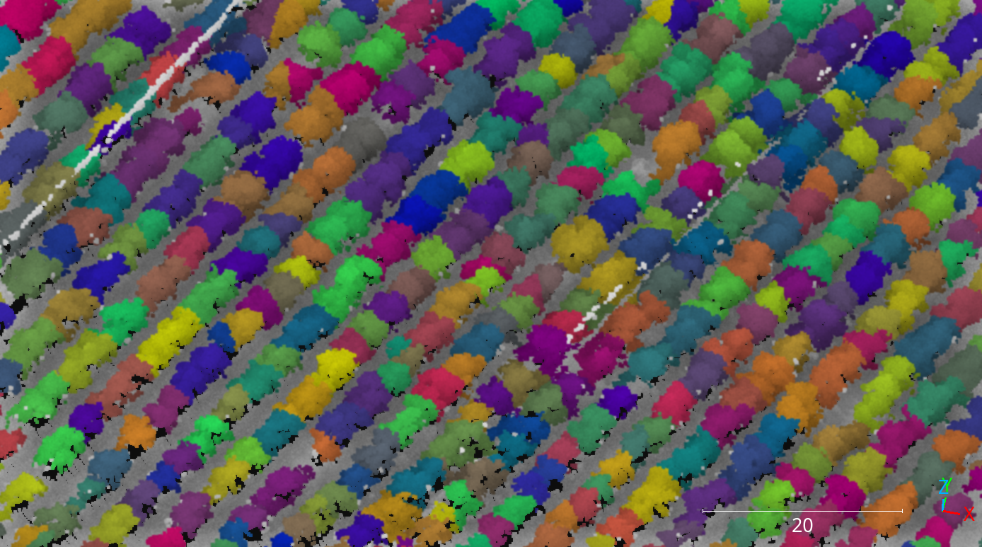
Figure representing avocado cluster. — Visualization of the avocado clusters computed through the bivariate critical clustering algorithm with the region growing strategy.

Post-processing

Once clusters are available, it might be useful to apply some post-processing to derive useful information from them. That is what post-processing components aim to do. They can be defined in the "post_clustering" list. The execution will start by the first component in the list and will end at the last one, i.e., it is sequential with respect to the order in the list.

ClusterEnveloper

The ClusterEnveloper can be used to find the geometry enclosing the points. Envelopes often support the estimation of the enclosed volume. They can be exported to output files. The JSON below shows how to define a cluster enveloper post-processor inside the post-processing pipeline of a clusterer.

"post_clustering": [
    {
        "post-processor": "ClusterEnveloper",
        "envelopes": [
            {
                "type": "AlignedBoundingBox",
                "compute_volume": true,
                "output_path": "*/aabbs.csv",
                "separator": ","
            },
            {
                "type": "BoundingBox",
                "compute_volume": true,
                "output_path": "*/bboxes.csv",
                "separator": ","
            }
        ]
    }
]

The JSON above defines a ClusterEnveloper that will compute the axis-aligned bounding box and also the oriented bounding box. The volume will be computed for each envelope and they will be exported to a CSV file. More concretely, each row in the CSV will contain three coordinates representing a vertex, an integer representing the cluster label, and the estimated volume. All the values will be separated by ,.

Arguments

– envelopes

List of envelopes that must be computed by the ClusterEnveloper

– type

The type of the envelope, it can be "AxisAlignedBoundingBox" or "BoundingBox" (the edges of the last one are not necessarily parallel to the vectors of the canonical basis).

– compute_volume

Flag to specify whether to compute the volume enclosed by the envelope (true) or not (false).

– output_path

The path where the envelope’s data will be exported (typically in CSV format).

– separator

The separator to be used in the output CSV file.

ClusterMarker

The ClusterMarker can be used to compute a point for each cluster to represent it. These points can be exported as CSV files or shapefiles. The JSON below shows how to define a cluster marker post-processor inside the post-processing pipeline of a clusterer.

"post_clustering": [
    {
        "post-processor": "ClusterMarker",
        "strategy": "centroid",
        "proj_str": null,
        "epsg": 32630,
        "output_path": "*/marks.shp",
        "nthreads": -1
    }
]

The JSON above defines a ClusterMarker that will compute the centroid for each cluster as a marker. The output will be exported in the EPSG:32630 CRS to a shapefile called marks.shp. The computations will be carried out using all the cores available in the system.

Arguments

– strategy: The strategy that must be used to compute the markers. Supported strategies are "centroid", (see ClusterMarker.compute_cluster_centroid()), "midrange" (see ClusterMarker.compute_cluster_midrange()), "medianoid" (see ClusterMarker.compute_cluster_medianoid()), "medoid" (see ClusterMarker.compute_cluster_medoid()), and "geometric_median" (see ClusterMarker.compute_cluster_geometric_median()).
– proj_str: The coordinate reference system specified as a projection string (proj).
– epsg: Can be optionally used to specified the CRS following the European Petroleum Survey Groups (EPSG) standard format.
– nthreads: The number of threads that must be used for the parallel computations. Note that -1 means using as many threads as available cores.
– output_path: The output path where the markers must be written. Note that if the extension is .shp, then the output will be written as a shapefile. Otherwise, it will be written as an ASCII CSV file.

ClusterSelector

The ClusterSelector can be used to discard those clusters that do not satisfy satisfy some given criteria. It consists of a list of filters that check some given relationals and either preserve or discard those clusters that satisfy them. The JSON below shows how to define a cluster enveloper post-processor inside the post-processing pipeline of a clusterer.

"post_clustering": [
    {
        "post-processor": "ClusterSelector",
        "filters": [
          {
            "attribute": "number_of_points",
            "relational": "greater_than_or_equal_to",
            "target": 256,
            "action": "preserve"
          },
          {
            "attribute": "surface_area",
            "relational": "less_than",
            "target": 1,
            "action": "discard"
          },
          {
            "attribute": "z_length",
            "relational": "less_than",
            "target": 3,
            "action": "discard"
          }
        ]
    }
]

The JSON above defines a ClusterSelector that will preserve only the clusters with at least \(256\) points and discard those whose convex hull has a surface area less than \(1\) meter or whose length along the \(z\)-axis is below the \(3\) meters.

Arguments

– filters

The list of filters based on relational conditions to decide whether to preserve or discard those clusters who satisfy them.

– attribute: The attribute involved in the relational condition as the left-hand side. Supported attributes are "number_of_points", "surface_area", "volume", "surface_density", "volume_density", "x_length", "y_length" and "z_length". Their description can be read in the documentation of ClusterSelector.
– relational: The relational governing the condition. Supported relationals are "not_equals" \(x \neq y\), "equals" \(x = y\), "less_than" \(x < y\), "less_than_or_equal_to" \(x \leq y\), "greater_than" \(x > y\), "greater_than_or_equal_to" \(x \geq y\), "in" \(x \in S\), "not_in" \(x \notin S\), and "inside" \(x \in [a, b] \subset \mathbb{R}\).
– target: The right-hand side of the relational condition.
– action: Whether to "preserve" or "discard" the clusters that satisfy the relational condition.

Decorators

Furthest point sampling decorator

The FPSDecoratorTransformer can be used to decorate a data clusterer such that the computations can take place in a transformed space of reduced dimensionality. Typically, the domain of a clustering is the entire point cloud, let us say \(m\) points. When using a FPSDecoratedClusterer this domain will be transformed to a subset of the original point cloud with \(R\) points, such that \(m \geq R\). Decorating a clusterer with this decorator can be useful to reduce its execution time.

{
    "clustering": "fpsdecorated",
    "fps_decorator": {
        "num_points": "m/10",
        "fast": true,
        "num_encoding_neighbors": 1,
        "num_decoding_neighbors": 1,
        "release_encoding_neighborhoods": false,
        "threads": 16,
        "representation_report_path": null
    },
    "decorated_clusterer": {
        "clustering": "dbscan",
        "cluster_name": "cluster_wood",
        "precluster_name": "Prediction",
        "precluster_domain": [1],
        "min_points": 200,
        "radius": 3.0,
        "post_clustering": [
            {
                "post-processor": "ClusterEnveloper",
                "envelopes": [
                    {
                        "type": "AlignedBoundingBox",
                        "compute_volume": true,
                        "output_path": "*/aabbs.csv",
                        "separator": ","
                    },
                    {
                        "type": "BoundingBox",
                        "compute_volume": true,
                        "output_path": "*/bboxes.csv",
                        "separator": ","
                    }
                ]
            }
        ]
    }
}

Arguments

– fps_decorator

The specification of the furthest point sampling (FPS) decoration carried out through the FPSDecoratorTransformer.

– num_points: The target number of points \(R\) for the transformed point cloud. It can be an integer or an expression that will be evaluated with \(m\) representing the number of points of the original point cloud, e.g., "m/2" will downscale the point cloud to half the number of points.
– fast: Whether to use exact furthest point sampling (false) or a faster stochastic approximation (true).
– num_encoding_neighbors: How many closest neighbors in the original point cloud are considered for each point in the transformed point cloud to reduce from the original space to the transformed one.
– num_decoding_neighbors: How many closest neighbors in the transformed point cloud are considered for each point in the original point cloud to propagate back from the transformed space to the original one.
– release_encoding_neighborhoods: Whether the encoding neighborhoods can be released after computing the transformation (true) or not (false). Releasing these neighborhoods means the FPSDecoratorTransformer.reduce() method must not be called, otherwise errors will arise. Setting this flag to true can help saving memory when needed.
– threads: The number of parallel threads to consider for the parallel computations. Note that -1 means using as many threads as available cores.
– representation_report_path: Where to export the transformed point cloud. In general, it should be null to prevent unnecessary operations. However, it can be enabled (by given any valid path to write a point cloud file) to visualize the points that are seen by the data miner.

– decorated_clusterer

A typical clustering specification. See the DBScan clusterer for an example.

Minimum distance decimator decorator

The MinDistDecimatorDecorator can be used to decorate a clusterer such that the computations can take place in a transformed space of reduced dimensionality. Typically, the domain of a clusterer is the entire point cloud, let us say \(m\) points. When using a MinDistDecoratedClusterer this domain will be transformed to a subset of the original point cloud with \(R \leq m\) points. This representation is achieved by assuring that no point is closer to its closest neighbor than a given minimum distance threshold. Decorating a clusterer with this decorator can be useful to reduce its execution time.

{
    "clustering": "MinDistDecorated",
    "mindist_decorator": {
        "min_distance": 0.3,
        "num_encoding_neighbors": 1,
        "num_decoding_neighbors": 1,
        "release_encoding_neighborhoods": false,
        "threads": -1,
        "representation_report_path": null
    },
    "decorated_clusterer": {
        "clustering": "dbscan",
        "cluster_name": "bunny",
        "precluster_name": "classification",
        "min_points": 3,
        "radius": 3.0
    }
}

Arguments

– mindist_decorator: See the minimum distance decorated miner documentation about arguments .
– decorated_clusterer: A typical clustering specification. See the DBScan clusterer for an example.