Data mining
Data miners are components that receive an input point cloud and extract
features characterizing it, typically in a point-wise fashion.
Data miners (Miner) can be included inside pipelines to generate
features that can later be used to train a machine learning model to perform
a classification or regression task on the points.
Geometric features miner
The GeomFeatsMiner uses
Jakteristics
as backend to compute point-wise geometric features. The point-wise features
are computed considering spherical neighborhoods of a given radius. The JSON
below shows how to define a GeomFeatsMiner.
{
    "miner": "GeometricFeatures",
    "in_pcloud": null,
    "out_pcloud": null,
    "radius": 0.3,
    "fnames": ["linearity", "planarity", "surface_variation", "verticality", "anisotropy"],
    "frenames": ["linearity_r0_3", "planarity_r0_3", "surface_variation_r0_3", "verticality_r0_3", "anisotropy_r0_3"],
    "nthreads": -1
}
The JSON above defines a GeomFeatsMiner that computes the linearity,
planarity, surface variation, verticality, and anisotropy geometric features
considering a \(30\,\mathrm{cm}\) radius for the spherical neighborhood.
The computed features will be named from the feature names and the neighborhood
radius. Parallel regions will be computed using all available threads.
Arguments
- –
in_pcloud When the data miner is used outside a pipeline, this argument can be used to specify which point cloud must be loaded to compute the geometric features on it. In pipelines, the input point cloud is considered to be the point cloud at the current pipeline’s state.
- –
out_pcloud When the data miner is used outside a pipeline, this argument can be used to specify where to write the output point cloud with the computed geometric features. Otherwise, it is better to use a Writer to export the point cloud after the data mining.
- –
radius The radius for the spherical neighborhood.
- –
fnames The list with the names of the features that must be computed. Supported features are:
["eigenvalue_sum", "omnivariance", "eigenentropy", "anisotropy", "planarity", "linearity", "PCA1", "PCA2", "surface_variation", "sphericity", "verticality"]- –
frenames The list of names for the generated features. If it is not given, then the generated features will be automatically named.
- –
nthreads How many threads use to compute parallel regions. The value -1 means as many threads as supported in parallel (typically including virtual cores).
Output
The figure below represents the planarity and verticality features mined for a spherical neighborhood with \(30\,\mathrm{cm}\) radius. The point cloud for this example corresponds to the Paris point cloud from the Paris-Lille-3D dataset.
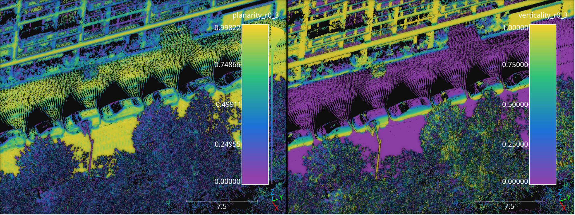
Visualization of the planarity (left) and verticality (right) computed in the Paris point cloud from the Paris-Lille-3D dataset using spherical negibhorhoods with \(30\,\mathrm{cm}\) radius.
Geometric features miner ++
The GeomFeatsMinerPP represents an improved version with better
workload balancing and more geometric features compared to the
GeomFeatsMiner. The main improvements are a flexible neighborhood
definition that includes spheres, cylinders, rectangular prisms, and k-nearest
neighbors (knn); the possibility to choose between singular value decomposition
SVD and principal component analysis (PCA) as the factorization strategy
for the structure space matrix representing the neighborhood; a Taubin method
for improved quadric fitting, and the inclusion
of roughness and second order geometric features like the mean and Gaussian
curvatures. The JSON below shows how to define a GeomFeatsMinerPP.
{
    "miner": "GeometricFeaturesPP",
    "first_order_strategy": "pca",
    "second_order_strategy": "taubin_bias",
    "idw_p": 2,
    "idw_eps": 11,
    "foc_K": 0,
    "foc_sigma": 3.14159265358979323846264338327950288419716939937510,
    "neighborhood": {
      "type": "sphere",
      "radius": 33,
      "k": 1024,
      "lower_bound": 0,
      "upper_bound": 0
    },
    "fnames": [
        "linearity", "planarity", "sphericity", "surface_variation", "omnivariance", "anisotropy",
        "eigenentropy", "normalized_eigenentropy", "eigenvalue_sum", "roughness",
        "esval3", "full_eigen_index", "gauss_curv_full", "mean_curv_full", "full_quad_dev",
        "full_abs_algdist", "full_sq_algdist", "full_laplacian", "full_mean_qdev", "full_gradient_norm",
        "full_eigensum", "full_eigenentropy", "full_normalized_eigenentropy", "full_omnivariance",
        "full_hypersphericity", "full_hyperanisotropy", "full_spectral", "full_frobenius", "full_schatten",
        "full_linear_norm", "full_cross_norm", "full_square_norm", "full_abs_bias",
        "full_maxcurv", "full_mincurv", "full_maxabscurv", "full_minabscurv",
        "full_umbilic_dev", "full_rmsc", "full_umbilicality", "full_gauss_umbilicality", "full_shape_index",
        "full_min_eigenval", "saddleness", "minpg", "maxpg", "bipgnorm",
        "normalized_minpg", "normalized_maxpg", "normalized_bipgnorm",
        "gradient_axis_curv", "normalized_gac", "full_normalized_gac"
      ],
    "frenames": [
        "linear_r33", "planar_r33", "spheric_r33", "surfvar_r33", "omnivar_r33", "anisotropy_r33",
        "eigentropy_r33", "eigsum_r33", "roughness_r33", "esval3_r33", "eigidx_r33",
        "full_gauss_r33", "full_mean_r33", "full_qdev_r33", "abs_algdist_r33", "sq_algdist_r33",
        "laplacian_r33", "full_meanqdev_r33", "full_gradnorm_r33",
        "full_eigsum_r33", "full_eigentropy_r33", "full_omnivar_r33", "hyperspher_r33", "hyperanisotropy_r33",
        "spectral_r33", "frobenius_r33", "schatten_r33",
        "linear_norm_r33", "cross_norm_r33", "square_norm_r33", "full_abs_bias_r33",
        "maxcurv_r33", "mincurv_r33", "maxabscurv_r33", "minabscurv_r33",
        "umbilic_dev_r33", "rmsc_r33", "umbilicality_r33", "gumbilicality_r33", "shape_index_r33",
        "full_min_eigval_r33", "saddleness_r33", "minpg_r33", "maxpg_r33", "bipgnorm_r33",
        "normalized_minpg_r33", "normalized_maxpg_r33", "normalized_bipgnorm_r33",
        "gac_r33", "normalized_gac_r33", "fnormed_gc_r33"
    ],
    "non_degenerate_eigenthreshold": 0.00001,
    "tikhonov_parameter": 0.0000001,
    "nthreads": -1
}
The JSON above defines a GeomFeatsMinerPP that computes the linearity,
planarity, sphericity, surface variation, omnivariance, anisotropy,
eigenentropy, sum of eigenvalues, roughness, gaussian curvature, mean curvature,
quadratic deviation, Laplacian, shape index, Gaussian umbilicality, and many more
on a spherical neighborhood with \(33\,\mathrm{mm}\) radius. The computed
features will be named from the feature names and the
neighborhood radius. The computations will be carried in parallel using all the
available cores. The eigenthreshold to detect degenerate cases for quadric
fitting is set to \(10^{-5}\), the parameter for the Tikhonov regularization
is set to \(10^{-7}\). The first order geometric descriptors are computed
with PCA, the second order geometric descriptors use a biased quadric model
fit with Taubin method and apply Inverse Distance Weighting (IDW) with
\(p=2\) and \(\epsilon=11\). There is no Fibonacci orthodromic
correction of the IDW weights because "foc_K": 0.
Arguments
- –
first_order_strategy The strategy for the linear fit. Whether
"svd"to consider the singular values and singular vectors from \(X = \pmb{U}\pmb{\Sigma}\pmb{V}^{\intercal} \in \mathbb{R}^{m \times 3}\) for a 3D neighborhood of m points, where the columns of \(\pmb{V} \in \mathbb{R}^{3 \times 3}\) are the singular vectors and \(\operatorname{diag}\left(\pmb{\Sigma}\right) \in \mathbb{R}^{3}\) gives the singular values; or"pca"to consider the eigenvalues and eigenvectors of \(\pmb{X}^{\intercal}\pmb{X}\). For"svd"the matrix \(\pmb{X}\) is centered and for"pca"it is centered and divided by \(m-1\) to be a covariance matrix. The recommended approach is"pca".- –
second_order_strategy The strategy for the quadric fit. It can be either
"svd","pca","taubin"to fit an unbiased quadric \(g(x, y, z) = w_1x + w_2y + w_3z + w_4xy + w_5xz + w_6yz + w_7x^2 + w_8y^2 + w_9z^2\) or"svd_bias","pca_bias","taubin_bias"to fit a biased quadric \(g(x, y, z) = w_1x + w_2y + w_3z + w_4xy + w_5xz + w_6yz + w_7x^2 + w_8y^2 + w_9z^2 + w_{10}\) . The recommended approach is"taubin_bias", yet faster approaches like"pca"or"pca_bias"might be preferred if only second order geometric descriptors based on quadric eigenvalues will be considered. For the computation of second order geometric descriptors involving curvatures the Taubin method provides a more stable solution incorporating a second matrix obtained by summing the outer products of the partial derivatives of the polynomial coordinates.- –
idw_p The \(p\) parameter governing the Inverse Distance Weighting (IDW) strategy to weight the contribution of each point in the neighborhood to the quadric fit. If \(p=0\) no IDW will be applied at all.
- –
idw_eps The \(\epsilon\) parameter governing the Inverse Distance Weighting (IDW). It represents the min accepted value so distances below it will be automatically replaced.
- –
foc_K The number of points in the spherical Fibonacci support. The greater the better but it will lead to higher execution times (i.e., it increases the computational cost).
- –
foc_sigma The hard cut threshold for the Fibonacci orthodromic correction between a point in a centered neighborhood \(\pmb{x}_{j*} \in \mathbb{R}^{3}\) and a point from the Fibonacci support \(\pmb{q}_{k*} \in \mathbb{R}^{3}\).
\[\omega(\pmb{x}_{j*}, \pmb{q}_{k*}) = \max \left\{ 0, \sigma - \arccos\left(\dfrac{ \langle\pmb{x}_{j*}, \pmb{q}_{k*}\rangle }{ \lVert\pmb{x}_{j*}\rVert } \right) \right\}\]See the C++ documentation for further mathematical details.
- –
non_degenerate_eigenthreshold The threshold to detect degenerated cases for the quadric fit depending on the min eigenvalue of the linear fit. When the min linear eigenvalue is below this threshold, the case is considered as degenerate. Recommended values for 32 bits decimal arithmetic are \(10^{-5}\) for the raw case (i.e., without smoothing and inverse distance weighting) and alternatively \(10^{-6}\) for cases with smoothing and inverse distance weighting. Note that degenerate cases are understood as planes with zero curvature when computing second order geometric descriptors.
- –
tikhonov_parameter Parameter governing the Tikhonov regularization. It is typically necessary on real data to assure the Cholesky decomposition (and any other similar operation) is numerically feasible. Recommended value for 32 bits decimal arithmetic is \(10^{-7}\).
- –
neighborhood The neighborhood definition.
- –
type Supported neighborhood types are
"cylinder","bounded_cylinder","sphere","rectangular2d","rectangular3d","knn2d","knn","boundedknn2d", and"boundedknn".- –
radius For neighborhoods with a single radius (e.g., spherical neighborhoods), it gives the radius. For neighborhoods with many radii (e.g., rectangular neighborhoods) it gives the first radius (typically along \(\pmb{e_1}\), i.e., \(x\)-axis). For bounded knn neighborhoods the radius also gives the radial bound, i.e., the max distance to consider a neighbor as near.
- –
k The number of neighbors for knn neighborhoods.
- –
lower_bound The lower bound along the vertical axis of a cylindrical neighborhood or a rectangular 2D neighborhood. Also, the length along \(\pmb{e_2}\), i.e., \(y\)-axis, for 3D rectangular neighborhoods.
- –
upper_bound The upper bound along the vertical axis of a cylindrical neighborhood or a rectangular 3D neighborhood. Also, the length along \(\pmb{e_3}\), i.e., \(z\)-axis, for 3D rectangular neighborhoods.
- –
- –
fnames The list with the names of the features that must be computed. Supported features are:
["linearity", "planarity", "sphericity", "surface_variation", "roughness", "verticality", "altverticality", "sqverticality", "horizontality", "sqhorizontality", "eigenvalue_sum", "omnivariance", "eigenentropy", "anisotropy", "PCA1", "PCA2", "number_of_neighbors", "fom", "nx", "ny", "nz", "esval1", "esval2", "esval3", "gauss_curv_full", "mean_curv_full", "full_quad_dev", "full_abs_algdist", "full_sq_algdist", "full_laplacian", "full_mean_qdev", "full_gradient_norm", "full_eigensum", "full_eigenentropy", "full_omnivariance", "full_hypersphericity", "full_hyperanisotropy", "full_spectral", "full_frobenius", "full_schatten", "full_coeff_norm", "full_linear_norm", "full_cross_norm", "full_square_norm", "full_deg2_norm", "full_nlinear_norm", "full_ncross_norm", "full_nsquare_norm", "full_ndeg2_norm", "full_bias_term", "full_abs_bias", "full_maxcurv", "full_mincurv", "full_maxabscurv", "full_minabscurv", "full_umbilic_dev", "full_rmsc", "full_umbicality", "full_gauss_umbilicality", "full_shape_index", "full_eigen_index", "full_min_eigenval", "full_max_eigenval", "minpg", "maxpg", "avg", "normalized_minpg", "normalized_maxpg", "normalized_avg", "saddleness", "absolute_hg", "hgnorm", "normalized_hgn", "bipgnorm", "normalized_bipgnorm", "gradient_axis_curv", "normalized_gac", "full_normalized_gac", "hessian_frobenius", "hessian_absdet", "full_abs_quadraticity"]- –
frenames The list of names for the generated features. If it is not given, then the generated features will be automatically named.
- –
nthreads How many threads use to compute parallel regions. The value -1 means as many threads as supported in parallel (typically including virtual cores).
Output
The figure below represents the references (blue for vessel and red for
aneurysm), and some second order geometric descriptors like the linear norm,
shape index, and Gaussian umbilicality. The point cloud for this example was
generated by merging four different aneurysms from the
IntrA dataset
which can be downloaded from
Google drive.
Note that the point clouds were smoothed using a
SimpleStructureSmotherPP (see
Simple structure smoother ++ documentation
) with IDW strategy using \(p=1\), \(\epsilon=3\), and a spherical
neighborhood with a radius of \(11\;\mathrm{mm}\).
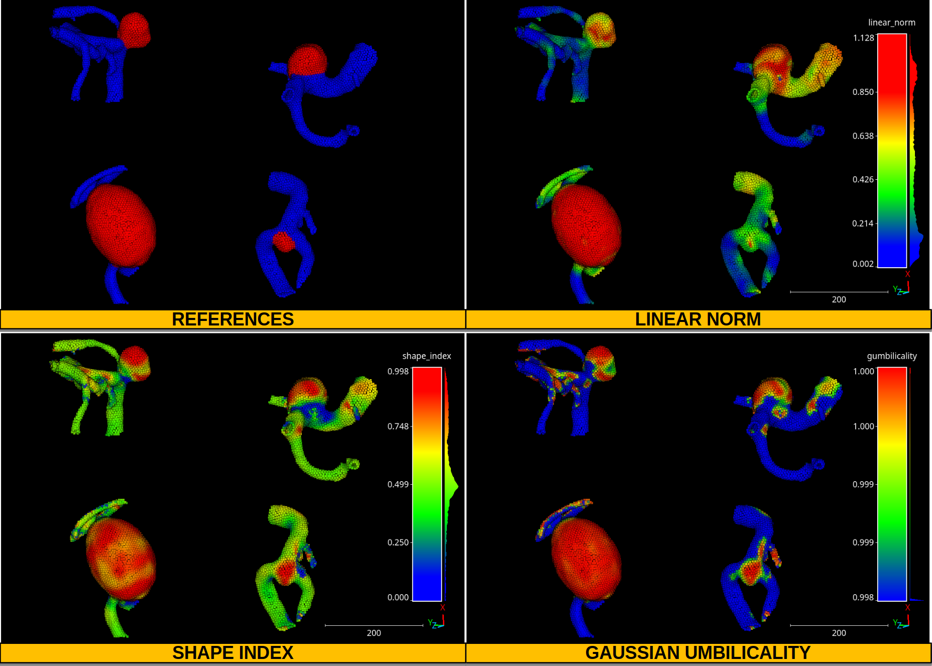
Visualization of four aneurysms. Vessel points are represented in blue, aneurysms in red. The color maps represent the distribution of the linear norm, the shape index, and the Gaussian umbilicality.
Height features miner
The HeightFeatsMiner supports the computation of height-based
features. These features assume that the \(z\) axis corresponds to the
vertical axis and derive features depending on the \(z\) values of
many neighborhoods. The neighborhoods are centered on support points. Finally,
each point in the point cloud will take the features from the closest support
point. The JSON below shows how to define a HeightFeatsMiner:
{
    "miner": "HeightFeatures",
    "support_chunk_size": 50,
    "support_subchunk_size": 10,
    "pwise_chunk_size": 1000,
    "nthreads": 12,
    "neighborhood": {
        "type": "Rectangular2D",
        "radius": 50.0,
        "separation_factor": 0.35
    },
    "outlier_filter": null,
    "fnames": ["floor_distance", "ceil_distance"]
}
The JSON above defines a HeightFeatsMiner that computes the distance
to the floor (lowest point) and to the ceil (highest point). It considers
a rectangular neighborhood for the support points with side length
\(50 \times 2 = 100\) meters. Not outlier filter is applied.
Arguments
- –
support_chunk_size The number of support points per chunk for parallel computations.
- –
support_subchunk_size The number of simultaneous neighborhoods considered when computing a chunk. It can be used to prevent memory exhaustion scenarios.
- –
pwise_chunk_size The number of points per chunk when computing the height features for the points in the point cloud (not the support points).
- –
nthreads How many threads must be used for parallel computations (-1 means as many threads as available cores).
- –
neighborhood The neighborhood definition. The type can be either
"Rectangular2D"(the radius describes half of the side) or"Cylinder"(the radius describes the disk of the cylinder). The separation factor governs the separation of the support points considering the radius. Note that if separation factor is set to zero, then the height features will be computed on a point-wise fashion. SeeGridSubsamplingPreProcessorfor more details.- –
outlier_filter The strategy to filter outlier points (it can be None). Supported strategies are
"IQR"and"stdev". The"IQR"strategy considers the interquartile range and discards any height value outside \([Q_1-3\mathrm{IQR}/2, Q_3+3\mathrm{IQR}/2]\). The"stdev"strategy discards any height value outside \([\mu - 3\sigma, \mu + 3\sigma]\) where \(\mu\) is the mean and \(\sigma\) is the standard deviation.- –
fnames The name of the height features that must be computed. Supported height features are:
["floor_coordinate", "floor_distance", "ceil_coordinate",
"ceil_distance", "height_range", "mean_height", "median_height",
"height_quartiles", "height_deciles", "height_variance",
"height_stdev", "height_skewness", "height_kurtosis"]
Output
The figure below represents the floor distance mined for a spherical Rectangular2D neighborhood with \(50\) meters radius. The point cloud from this example corresponds to the March2018 validation point cloud from the Hessigheim dataset.
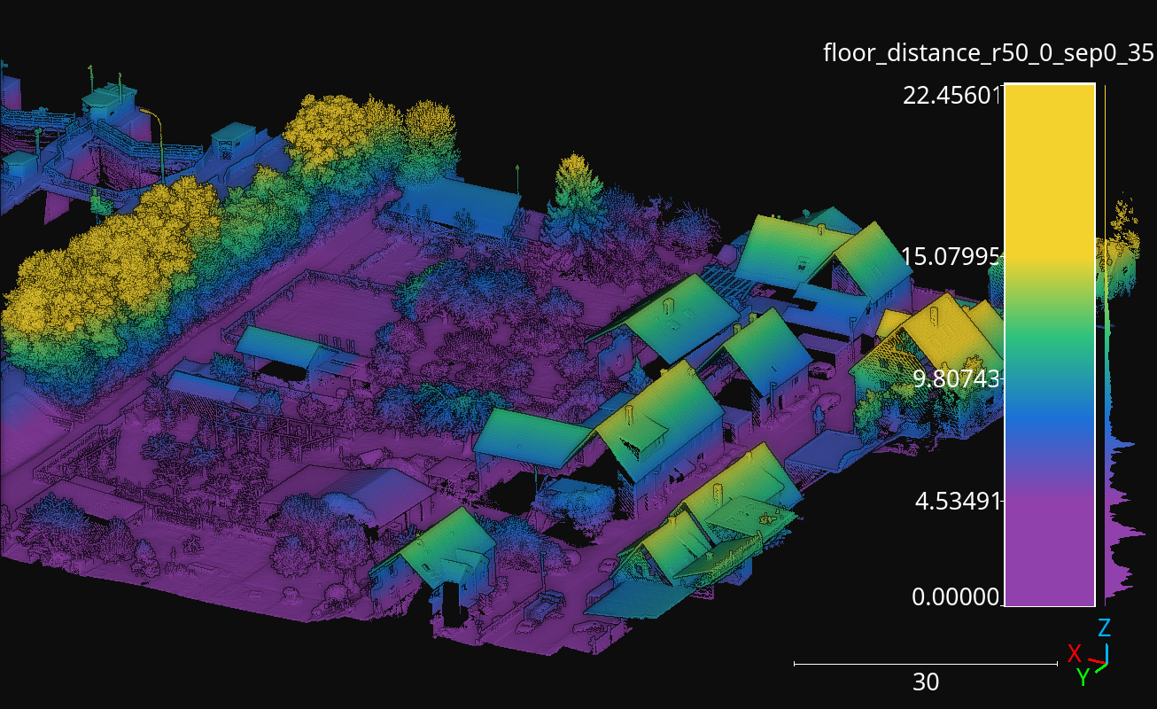
Visualization of the floor distance height feature computed for the Hessigheim March2018 validation point cloud using using a Rectangular2D neighborhood with \(50\,\mathrm{m}\) radius.
Height features miner ++
The HeightFeatsMinerPP represents an improved version with better
computational efficiency than the HeightFeatsMiner. Using this
component inside pipelines can be done with the JSON specification described
for the Height features miner. The only
difference is that "miner" argument must be set to "HeightFeaturesPP"
instead of "HeightFeatures".
HSV from RGB miner
The HSVFromRGBMiner can be used when red, green, and blue color channels
are available for the points in the point cloud. It will generate the
corresponding hue (H), saturation (S), and value (V) components derived from
the available RGB information. The JSON below shows how to define a
HSVFromRGBMiner:
{
    "miner": "HSVFromRGB",
    "hue_unit": "radians",
    "frenames": ["HSV_Hrad", "HSV_S", "HSV_V"]
}
The JSON above defines a HSVFromRGBMiner that computes the HSV
representation of the original RGB color components.
Arguments
- –
hue_unit The unit for the hue (H) component. It can be either
"radians"or"degrees".- –
frenames The name for the output features. If not given, they will be
["HSV_H", "HSV_S", "HSV_V"]by default.
Output
The figure below represents the saturation (S) computed for the March2018 validation point cloud from the Hessigheim dataset.
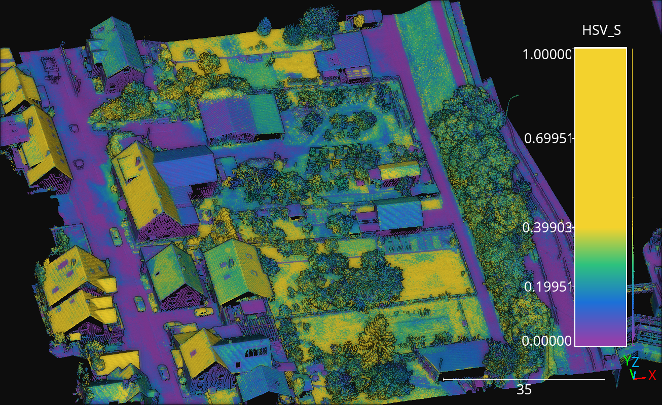
Figure representing the saturation (S) in the March2018 validation point cloud of the Hessigheim dataset.
Smooth features miner
The SmoothFeatsMiner can be used to derive smooth features from
already available features. The mean, weighted mean, and Guassian
Radial Basis Function (RBF) strategies can be used for this purpose. The JSON
below shows how to define a SmoothFeatsMiner:
{
    "miner": "SmoothFeatures",
    "nan_policy": "propagate",
    "chunk_size": 1000000,
    "subchunk_size": 1000,
    "neighborhood": {
        "type": "sphere",
        "radius": 0.25
    },
    "input_fnames": ["Reflectance", "HSV_Hrad", "HSV_S", "HSV_V"],
    "fnames": ["mean"],
    "nthreads": 12
}
The JSON above defines a SmoothFeatsMiner that computes the smooth
reflectance, and HSV components considering a spherical neighborhood with
\(25\,\mathrm{cm}\) radius. The strategy consists of computing the mean
value for each neighborhood. The computations are run in parallel using 12
threads.
Arguments
- –
nan_policy It can be
"propagate"(default) so NaN features will be included in computations (potentially leading to NaN smooth features). Alternatively, it can be"replace"so NaN values are replaced with the feature-wise mean for each neighborhood. However, using"replace"leads to longer executions times. Therefore,"propagate"should be used always that NaN handling is not necessary.- –
chunk_size How many points per chunk must be considered for parallel computations.
- –
subchunk_size How many neighborhoods per iteration must be considered when computing a chunk. It can be useful to prevent memory exhaustion scenarios.
- –
neighborhood The definition of the neighborhood to be used. Supported neighborhoods are
"knn"(for which a"k"value must be given),"sphere"(for which a"radius"value must be given), and"cylinder"(the"radius"refers to the disk of the cylinder).
- –
weighted_mean_omega The \(\omega\) parameter for the weighted mean strategy (see
SmoothFeatsMinerfor a description of the maths).
- –
gaussian_rbf_omega The \(\omega\) parameter for the Gaussian RBF strategy (see
SmoothFeatsMinerfor a description of the maths).
- –
input_fnames The names of the features that must be smoothed.
- –
fnames The names of the smoothing strategies to be used. Supported strategies are
"mean","weighted_mean", and"gaussian_rbf".
- –
frenames The desired names for the generated output features. If not given, the names will be automatically derived.
- –
nthreads The number of threads to be used for parallel computations (-1 means as many threads as available cores).
Output
The figure below represents the smoothed saturation computed for two spherical neighborhoods with \(25\,\mathrm{cm}\) and \(3\,\mathrm{m}\) radius, respectively. The point cloud is the March2018 validation one from the Hessigheim dataset.
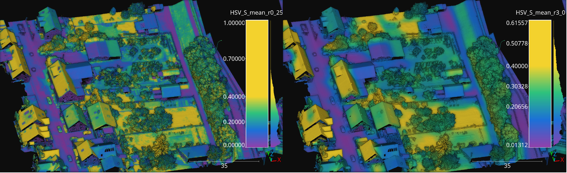
Figure representing the smoothed saturation for two different spherical neighborhoods with \(25\,\mathrm{cm}\) and \(3\,\mathrm{m}\) radius, respectively.
Smooth features miner ++
The class SmoothFeatsMinerPP can be used to derive smooth features
from already available features. It is similar to the
SmoothFeatsMiner class documented
above. The main difference is that the C++
version supports more neighborhood definitions like 2D and 3D rectangular
regions, 2D k-nearest neighbors, and bounded cylinders. The JSON below shows
how to define a SmoothFeatsMinerPP:
{
  "in_pcloud": [
    "/ext4/lidar_data/semantic3d/laz/domfountain_station1_xyz_intensity_RGB.laz"
  ],
  "out_pcloud": [
    "out/smooth_feats_pp/*"
  ],
  "sequential_pipeline": [
    {
        "miner": "FPSDecorated",
        "fps_decorator": {
            "num_points": "m/10",
            "fast": true,
            "num_encoding_neighbors": 1,
            "num_decoding_neighbors": 1,
            "release_encoding_neighborhoods": false,
            "threads": -1,
            "representation_report_path": "*repr.las"
        },
        "decorated_miner": {
            "miner": "SmoothFeaturesPP",
            "nan_policy": "replace",
            "neighborhood": {
                "type": "boundedcylinder",
                "radius": 0.3,
                "lower_bound": -0.45,
                "upper_bound": 0.45
            },
            "weighted_mean_omega": 0.01,
            "gaussian_rbf_omega": 0.1977,
            "input_fnames": ["intensity"],
            "fnames": ["mean", "weighted_mean", "gaussian_rbf"],
            "frenames": ["inten_meanpp", "inten_wmeanpp", "inten_grbfpp"],
            "nthreads": -1
        }
    },
    {
        "writer": "Writer",
        "out_pcloud": "*domfountain_station1_feats.las"
    }
  ]
}
The JSON above defines a SmoothFeatsMinerPP that computes the smooth
intensity considering a bounded cylinder with a disk of radius \(0.3\)
and discarding any point that is \(0.45\) below or above the center of the
neighborhood. Note that before applying the C++ data miner, a receptive field
is computed to speedup the computation even further.
Arguments
- –
nan_policy - –
neighborhood The definition of the neighborhood to be used. Supported neighborhoods are
"knn"(for which a"k"value must be given),"knn2d"(a k-nearest neighbor considering the \(x\) and \(y\) coordinates only),"sphere"(for which a"radius"value must be given),"cylinder"(the"radius"refers to the disk of the cylinder),"boundedcylinder"(the difference in the \(z\) coordinate with respect to the center point must be inside the given interval),"rectangular3d"(the"radius"defines the axis-wise half length for each edge), and"rectangular2d"(the rectangular region is defined for the \(x\) and \(y\) coordinates only).- –
weighted_mean_omega - –
gaussian_rbf_omega - –
input_fnames - –
fnames - –
frenames - –
nthreads
Output
The figure below represents the smoothed intensity computed in the bounded cylinder neighborhood defined in the example above. The left side of the figure represents the raw intensity, the right side the smoothed one (through a mean filter), so they can be compared. The data used in this example is the domfountain station1 point cloud from the Semantic3D dataset.
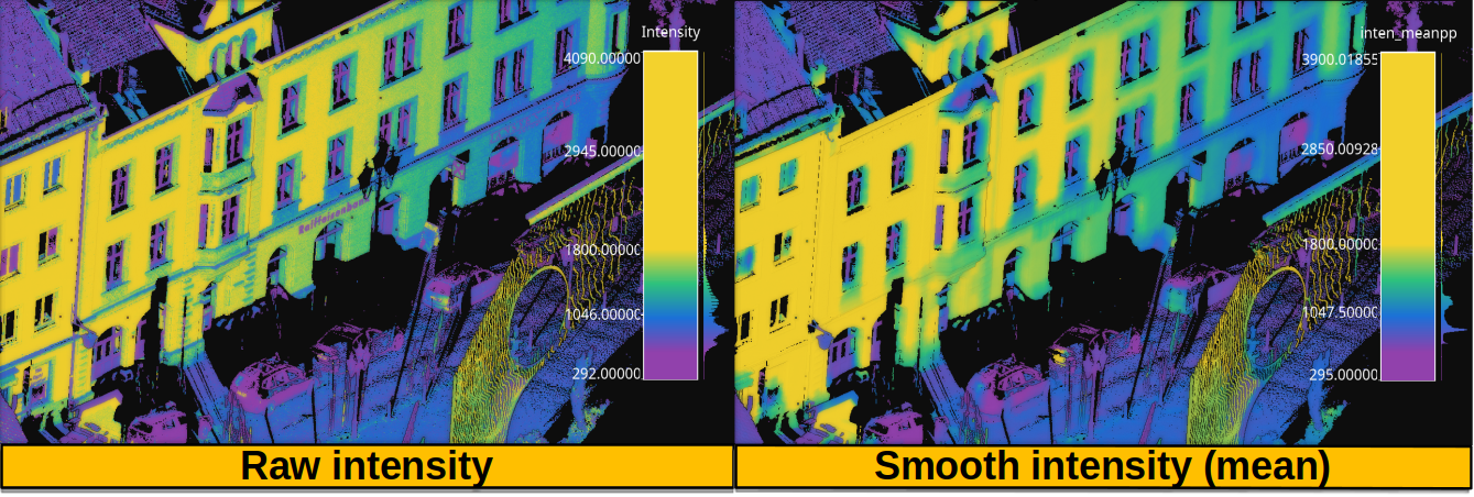
Figure representing the raw and smoothed (mean) intensity for a bounded cylindrical neighborhood with \(0.3\) radius and a \(0.45\) distance threshold for both the lower and upper bounds.
Recount miner
The RecountMiner can be used to derive features based on counting
the number of points. In doing so, many condition-based filters can be applied
to filter the points. Furthermore, the recount of points can be used as a
feature directly but also to derive the relative frequency, the surface density
(points per area), the volume density (points per volume), and the number of
vertical segments along a cylinder that contain at least one point passing the
filters. The JSON below shows how to define a RecountMiner:
{
    "miner": "Recount",
    "chunk_size": 100000,
    "subchunk_size": 1000,
    "nthreads": 16,
    "neighborhood": {
        "type": "cylinder",
        "radius": 3.0
    },
    "input_fnames": ["vegetation", "tower", "PointWiseEntropy", "Prediction"],
    "filters": [
        {
            "filter_name": "pdensity",
            "ignore_nan": false,
            "absolute_frequency": true,
            "relative_frequency": false,
            "surface_density": true,
            "volume_density": true,
            "vertical_segments": 0,
            "conditions": null
        },
        {
            "filter_name": "maybe_tower",
            "ignore_nan": true,
            "absolute_frequency": true,
            "relative_frequency": true,
            "surface_density": true,
            "volume_density": true,
            "vertical_segments": 0,
            "conditions": [
                {
                    "value_name": "tower",
                    "condition_type": "greater_than_or_equal_to",
                    "value_target": 0.333333

                }
            ]
        },
        {
            "filter_name": "as_tower",
            "ignore_nan": true,
            "absolute_frequency": true,
            "relative_frequency": true,
            "surface_density": true,
            "volume_density": true,
            "vertical_segments": 8,
            "conditions": [
                {
                    "value_name": "Prediction",
                    "condition_type": "equals",
                    "value_target": 4
                }
            ]
        },
        {
            "filter_name": "unsure_veg",
            "ignore_nan": true,
            "absolute_frequency": true,
            "relative_frequency": true,
            "surface_density": false,
            "volume_density": false,
            "vertical_segments": 0,
            "conditions": [
                {
                    "value_name": "Prediction",
                    "condition_type": "equals",
                    "value_target": 2
                },
                {
                    "value_name": "PointWiseEntropy",
                    "condition_type": "greater_than_or_equal_to",
                    "value_target": 0.1
                }
            ]
        },
        {
            "filter_name": "unsure_veg2",
            "ignore_nan": true,
            "absolute_frequency": true,
            "relative_frequency": true,
            "surface_density": false,
            "volume_density": false,
            "vertical_segments": 0,
            "conditions": [
                {
                    "value_name": "Prediction",
                    "condition_type": "equals",
                    "value_target": 2
                },
                {
                    "value_name": "vegetation",
                    "condition_type": "less_than",
                    "value_target": 0.666667
                }
            ]
        }
    ]
}
The JSON above defines a RecountMiner that computes features from
a previously classified point cloud. First, it computes the absolute frequency,
and the densities considering all points.
Then, it computes the frequencies and densities for
points whose likelihood to be a tower is equal to or above
\(0.\overline{3}\).
Afterwards, the frequencies, densities, and counts how many of eight vertical
segments contain at least one point, considering points predicted as tower.
Later, the frequencies for points that have been predicted as vegetation and
have a point-wise entropy greater than or equal to \(0.1\). Finally, the
frequencies for points predicted as vegetation with a likelihood less than
\(0.\overline{6}\).
Arguments
- –
chunk_size How many points per chunk must be considered for parallel computations.
- –
subchunk_size How many neighborhoods per iteration must be considered when computing a chunk. It can be useful to prevent memory exhaustion scenarios.
- –
nthreads The number of threads to be used for parallel computations (-1 means as many threads as available cores).
- –
neighborhood The definition of the neighborhood to be used. Supported neighborhoods are
"knn"(for which a"k"value must be given),"sphere"(for which a"radius"value must be given), and"cylinder"(the"radius"refers to the disk of the cylinder).
- –
input_fnames The names of the features to be considered when filtering the points.
- –
filters A list with all the filters that must be computed. One set of output features will be generated for each filter. Any filter can consist of none or many conditions. The filters can be defined such that:
- –
filter_name The name for the filter. It will be used to name the generated features.
- –
ignore_nan A flag governing how to handle nans. When set to
true, the filters will ignore points with nan values, i.e., they will not be counted.
- –
absolute_frequency Whether to generate a feature with the absolute frequency or raw count (
true) or not (false). The generated feature will be named by appending"_abs"to the filter name.
- –
relative_frequency Whether to generate a feature with the relative frequency (
true) or not (false). The generated feature will be named by appending"_rel"to the filter name.
- –
surface_density Whether to generate a feature by dividing the number of points by the surface area. The surface density is computed assuming the area of a circle. The radius of the circle will be the given one when using spherical or cylindrical neighborhoods but it will be derived as the distance between the center point and the furthest neighbor for knn neighborhoods. The generated feature will be named by appending
"_sd"to the filter name.
- –
volume_density Whether to generate a feature by dividing the number of points by the volume. The volume is computed assuming a sphere. The radius of the sphere will be the given one when using spherical neighborhoods but it will be derived as the distance between the center point and the furthest neighbor for knn neighborhoods. For cylindrical neighborhoods, a circle will be considered instead of the sphere, and the volume will be computed as the area of the circle along the boundaries of the vertical axis. The generated feature will be named by appending
"_vd"to the filter name.
- –
vertical_segments Whether to generate a feature by dividing the neighborhood into linearly spaced segments along the vertical axis and counting how many partitions contain at least one point satisfying the conditions. The generated feature will be named by appending
"_vs"to the filter name.
- –
conditions The list of conditions is a list of elements defined in the same way as the conditions of the Advanced input but without the
actionparameter, that is always assumed to be"preserve".
- –
Output
The generated output is a point cloud that includes the recount-based features.
Recount miner ++
The class RecountMinerPP can be used to derive recount features. It
is similar to the RecountMiner class documented
above. The main difference is that the C++ version
supports more neighborhood definitions like 2D and 3D rectangular regions,
2D k-nearest neighbors, and bounded cylinders. It also supports different
recounts like 2D and 3D sectors, rings, and radial boundaries (spherical
shells). The JSON below shows how to define a RecountMinerPP:
{
  "in_pcloud": [
    "/ext4/lidar_data/semantic3d/laz/domfountain_station1_xyz_intensity_rgb_smallcut.laz"
  ],
  "out_pcloud": [
    "out/vl3dpp/domfountain_station1_feats.las"
  ],
  "sequential_pipeline": [
    {
        "miner": "GeometricFeatures",
        "radius": 0.1,
        "fnames": ["linearity", "planarity"],
        "frenames": ["line_r0_1", "plan_r0_1"],
        "nthreads": 12
    },
    {
        "miner": "RecountPP",
        "nthreads": -1,
        "neighborhood": {
            "type": "cylinder",
            "radius": 0.1
        },
        "input_fnames": ["line_r0_1", "plan_r0_1", "classification"],
        "filters": [
            {
                "filter_name": "pdenspp",
                "ignore_nan": false,
                "absolute_frequency": true,
                "relative_frequency": false,
                "surface_density": false,
                "volume_density": true,
                "vertical_segments": 32,
                "conditions": null
            },
            {
                "filter_name": "cardenspp",
                "ignore_nan": true,
                "absolute_frequency": false,
                "relative_frequency": true,
                "surface_density": true,
                "volume_density": false,
                "vertical_segments": 0,
                "conditions": [
                    {
                        "value_name": "classification",
                        "condition_type": "equals",
                        "value_target": 7

                    }
                ]
            },
            {
                "filter_name": "plandenspp",
                "ignore_nan": true,
                "absolute_frequency": true,
                "relative_frequency": true,
                "surface_density": true,
                "volume_density": true,
                "vertical_segments": 0,
                "rings": 0,
                "radial_boundaries": 0,
                "sectors2D": 0,
                "sectors3D": 0,
                "conditions": [
                    {
                        "value_name": "plan_r0_1",
                        "condition_type": "greater_than_or_equal_to",
                        "value_target": 0.5

                    }
                ]
            },
            {
                "filter_name": "linedenspp",
                "ignore_nan": true,
                "absolute_frequency": true,
                "relative_frequency": true,
                "surface_density": true,
                "volume_density": true,
                "vertical_segments": 32,
                "rings": 8,
                "radial_boundaries": 8,
                "sectors2D": 16,
                "sectors3D": 32,
                "conditions": [
                    {
                        "value_name": "line_r0_1",
                        "condition_type": "greater_than_or_equal_to",
                        "value_target": 0.5

                    }
                ]
            }
        ]
    }
  ]
}
The JSON above defines a RecountMinerPP that computes a couple of
geometric features (linearity and planarity) for later computing recounts
based on those features. The first recount ("pdens") considers all the
points, the second recount considers all the points classified as car
("cardens"), the third one uses the planarity to select the points that have
at least a value \(0.5\), and the last one considers the points with a
linearity of at least \(0.5\).
Arguments
- –
nthreads - –
neighborhood - –
input_fnames - –
filters See Recount miner documentation.
–
filter_nameSee Recount miner documentation.–
ignore_nan: See Recount miner documentation.–
absolute_frequencySee Recount miner documentation.–
relative_frequencySee Recount miner documentation.–
surface_densitySee Recount miner documentation.–
volume_densitySee Recount miner documentation.–
vertical_segmentsSee Recount miner documentation.–
conditionsSee Recount miner documentation.–
ringsHow many concentric and linearly spaced rings (annuli) must be analyzed around the studied point. Non empty concentric rings will be counted. The generated feature will be named by appending"rin"to the filter name.–
radial_boundariesHow many concentric and linearly spaced radial boundaries (also known as spherical shells) must be analyzed around the studied point. Non empty spherical shells will be counted. The generated feature will be named by appending"rb"to the filter name.–
sectors2DHow many 2D sectors (on the horizontal plane, i.e., the one defined by the \(x\) and \(y\) coordinates) must be analyzed around the studied point. Non empty 2D sectors will be counted. The generated feature will be named by appending"st2"to the filter name.–
sectors3DHow many 3D sectors must be analyzed around the studied point. Non empty 3D sectors will be counted. The generated feature will be named by appending"st3"to the filter name.
Output
The generated output is a point cloud that includes the recount-based features. The figure below shows the linearity (left side) and the radial boundaries recount (right side) from the example above. The data used in this example is the domfountain station1 point cloud from the Semantic3D dataset.
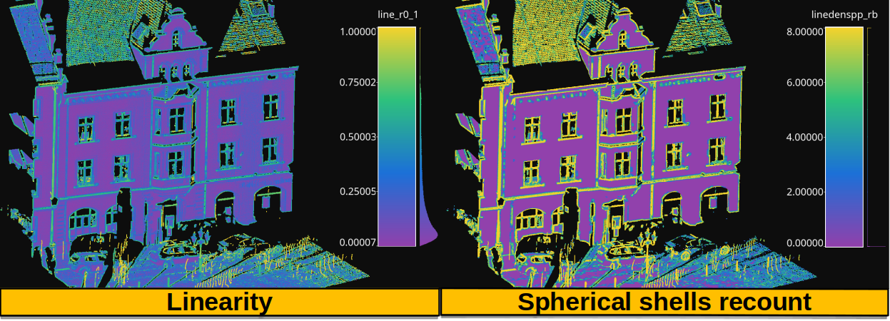
Figure representing the linearity computed from spherical neighborhoods of radius \(0.1\) in the left side. The right side shows the recount of spherical shells (radial boundaries) containing at least one point with a linearity greater than or equal to \(0.5\).
Take closest miner
The TakeClosestMiner can be used to derive features from another
point cloud. It works by defining a pool of point clouds such that the closest
neighbor between the input point cloud and any point cloud in the pool will be
considered. Then, the features for each point will be taken from its closest
neighbor.
{
    "miner": "TakeClosestMiner",
    "fnames": [
        "HSV_Hrad", "HSV_S", "HSV_V",
        "floor_distance_r50.0_sep0.35",
        "eigenvalue_sum_r0.3", "omnivariance_r0.3", "eigenentropy_r0.3",
        "anisotropy_r0.3", "planarity_r0.3", "linearity_r0.3",
        "PCA1_r0.3", "PCA2_r0.3",
        "surface_variation_r0.3", "sphericity_r0.3", "verticality_r0.3",
    ],
    "pcloud_pool": [
        "/home/point_clouds/point_cloud_A.laz",
        "/home/point_clouds/point_cloud_B.laz",
        "/home/point_clouds/point_cloud_C.laz"
    ],
    "distance_upper_bound": 0.1,
    "nthreads": 12
}
The JSON above defines a TakeClosestMiner that finds the features of
the closest point in a pool of three point clouds. Neighbors further than
\(0.1\,\mathrm{m}\) will not be considered, even if they are the closest
neighbor.
Arguments
- –
fnames The names of the features that must be taken from the closest neighbor in the pool.
- –
frenames An optional list with the name of the output features. When not given, the output features will be named as specified by
fnames.- –
y_default An optional value to be considered as the default label/class. If not given, it will be the max integer supported by the system.
- –
pcloud_pool A list with the paths to the point clouds composing the pool.
- –
distance_upper_bound The max distance threshold. Neighbors further than this distance will be ignored.
- –
nthreads The number of threads for parallel queries.
Output
The generated output is a point cloud where the features correspond to the
closest neighbor in the pool, assuming there is at least one neighbor that
is closer than the distance upper bound.
Decorators
Furthest point sampling decorator
The FPSDecoratorTransformer can be used to decorate a data miner such
that the computations can take place in a transformed space of reduced
dimensionality. Typically, the domain of a data miner is the entire point
cloud, let us say \(m\) points. When using a FPSDecoratedMiner
this domain will be transformed to a subset of the original point cloud with
\(R\) points, such that \(m \geq R\). Decorating a data miner with this
decorator can be useful to reduce its execution time.
{
    "miner": "FPSDecorated",
    "fps_decorator": {
        "num_points": "m/3",
        "fast": true,
        "num_encoding_neighbors": 1,
        "num_decoding_neighbors": 1,
        "release_encoding_neighborhoods": false,
        "threads": 16,
        "representation_report_path": "*/fps_repr/geom_r3_representation.las"
    },
    "decorated_miner": {
        "miner": "GeometricFeatures",
        "in_pcloud": null,
        "out_pcloud": null,
        "radius": 3.0,
        "fnames": ["linearity", "planarity", "surface_variation", "verticality", "anisotropy", "PCA1", "PCA2"],
        "frenames": ["linearity_r3", "planarity_r3", "surface_variation_r3", "verticality_r3", "anisotropy_r3", "PCA1_r3", "PCA2_r3"],
        "nthreads": 16
    }
}
Arguments
- –
fps_decorator The specification of the furthest point sampling (FPS) decoration carried out through the
FPSDecoratorTransformer.- –
num_points The target number of points \(R\) for the transformed point cloud. It can be an integer or an expression that will be evaluated with \(m\) representing the number of points of the original point cloud, e.g.,
"m/2"will downscale the point cloud to half the number of points.- –
fast Whether to use exact furthest point sampling (
false) or a faster stochastic approximation (true).
- –
num_encoding_neighbors How many closest neighbors in the original point cloud are considered for each point in the transformed point cloud to reduce from the original space to the transformed one.
- –
num_decoding_neighbors How many closest neighbors in the transformed point cloud are considered for each point in the original point cloud to propagate back from the transformed space to the original one.
- –
release_encoding_neighborhoods Whether the encoding neighborhoods can be released after computing the transformation (
true) or not (false). Releasing these neighborhoods means theFPSDecoratorTransformer.reduce()method must not be called, otherwise errors will arise. Setting this flag to true can help saving memory when needed.
- –
threads The number of parallel threads to consider for the parallel computations. Note that
-1means using as many threads as available cores.
- –
representation_report_path Where to export the transformed point cloud. In general, it should be
nullto prevent unnecessary operations. However, it can be enabled (by given any valid path to write a point cloud file) to visualize the points that are seen by the data miner.
- –
- –
decorated_miner A typical data mining specification. See the Geometric features miner for an example.
Minimum distance decimator decorator
The MinDistDecimatorDecorator can be used to decorate a data miner
such that the computations can take place in a transformed space of reduced
dimensionality. Typically, the domain of a data miner is the entire point
cloud, let us say \(m\) points. When using a MinDistDecoratedMiner
this domain will be transformed to a subset of the original point cloud with
\(R \leq m\) points. This representation is achieved by assuring that no
point is closer to its closest neighbor than a given minimum distance
threshold. Decorating a data miner with this decorator can be useful to reduce
its execution time.
{
    "miner": "MinDistDecorated",
    "mindist_decorator": {
        "min_distance": 0.02,
        "num_encoding_neighbors": 1,
        "num_decoding_neighbors": 1,
        "release_encoding_neighborhoods": false,
        "nthreads": -1,
        "representation_report_path": "*_representation.las"
    },
    "decorated_miner": {
        "miner": "GeometricFeaturesPP",
        "radius": 0.3,
        "fnames": [
            "linearity", "planarity", "surface_variation", "verticality", "anisotropy", "PCA1", "PCA2"
        ],
        "frenames": [
            "linearity_r0_3", "planarity_r0_3", "surface_variation_r0_3", "verticality_r0_3", "anisotropy_r0_3", "PCA1_r0_3", "PCA2_r0_3"
        ],
        "nthreads": -1
    }
}
Arguments
- –
mindist_decorator The specificaiton of the minimum distance decimation-based decorator carried out through
MinDistDecimatorDecorator.- –
min_distance The minimum distance threshold such that no pair of closest neighbors will be closer than this distance.
- –
num_encoding_neighbors See the num_encoding_neighbors documentation of FPSDecoratedMiner.
- –
num_decoding_neighbors See the num_decoding_neighbors documentation of FPSDecoratedMiner.
- –
release_encoding_neighborhoods See the release_encoding_neighborhoods documentation of FPSDecoratedMiner.
- –
threads
- –
representation_report_path See the representation_report_path documentation of FPSDecoratedMiner.
- –
- –
decorated_miner A typical data mining specification. See the Geometric features miner for an example.
Simple smoother decorator
The SimpleSmootherDecoratorTransformer can be used to decorate a data
miner such that the computations can take place in a transformed space where the
points are replaced by smooth versions with less abrupt changes. When using a
SimpleSmoothDecoratedMiner the data mining will be computed on the
smoothed representation of the point cloud. The C++ implementation accessible
through SimpleStructureSmootherPP enables the fast computation of
the many smoothing strategies.
{
    "miner": "SimpleSmoothDecorated",
    "simple_smoother_decorator": {
        "neighborhood": {
            "type": "sphere",
            "radius": 0.015,
            "k": 1
        },
        "strategy":{
            "type": "idw",
            "parameter": 2,
            "min_distance": 0.0015
        },
        "correction": null,
        "nthreads": -1,
        "representation_report_path": "*_smoothed.las"
    },
    "decorated_miner": {
        "miner": "GeometricFeaturesPP",
        "radius": 0.3,
        "fnames": [
            "linearity", "planarity", "surface_variation", "verticality", "anisotropy", "PCA1", "PCA2"
        ],
        "frenames": [
            "linearity_r0_3", "planarity_r0_3", "surface_variation_r0_3", "verticality_r0_3", "anisotropy_r0_3", "PCA1_r0_3", "PCA2_r0_3"
        ],
        "nthreads": -1
    }
}
Arguments
- –
simple_smoother_decorator The specification of the smoother decorator carried out through
SimpleSmootherDecoratorTransformer.- –
neighborhood The neighborhood specification. See
SimpleStructureSmootherPP.__init__()for further details.- –
type The type of neighborhood. Supported types are
"knn","knn2d","sphere"and"cylinder".- –
radius The radius for spherical and cylindrical neighborhoods.
- –
k The number of nearest neighbors in knn-based neighborhoods.
- –
- –
strategy The smoothing strategy. See
SimpleStructureSmootherPP.__init__()for further details.- –
type Either
"mean","idw"(inverse distance weighting), or"rbf"(Gaussian radial basis function).- –
parameter The parameter governing whether the inverse distance weighting or the Gaussian radial basis function equations.
- –
min_distance The min distance clip value to avoid division by zero when using inverse distance weighting.
- –
- –
correction The specification governing the Fibonacci correction. See
SimpleStructureSmootherPP.__init__()for further details.- –
K The \(K \in \mathbb{Z}_{>0}\) parameter governing how many points we must have in the Fibonacci support.
- –
sigma The cut threshold for the weighting function.
- –
- –
nthreads
- –
- –
decorated_miner A typical data mining specification. See the Geometric features miner for an example.