Machine learning
Machine learning was defined by Tom Mitchell in 1997 as computer programs that learn from experience \(E\) with respect to some task \(T\) and some performance measure \(P\). Here we will explain how machine learning can be used to solve tasks related to point clouds.
Note that applying machine learning models to point clouds requires point-wise
features because machine learning models will classify the points from the
features. The features can typically be specified through the fnames in
the JSON as a list of string where each string is the name of an attribute
in the input LAS/LAZ point cloud. Alternatively, features can also be mined
using the data mining methods in the VL3D framework. See
data mining documentation.
Models
Random forest classifier
The RandomForestClassificationModel can be used to solve point-wise
classification tasks. The random forest is an ensemble of decision trees such
that each individual decision tree is trained on a different random subset of
the training dataset. The final prediction of a random forest model for
classification is computed as the most frequent prediction considering all the
trees in the ensemble. In the VL3D framework,
scikit learn (sklearn)
is used as the backend for the random forest implementation. A
RandomForestClassificationModel can be defined as shown in the JSON
below:
{
    "train": "RandomForestClassifier",
    "fnames": ["AUTO"],
    "training_type": "base",
    "random_seed": null,
    "shuffle_points": false,
    "model_args": {
        "n_estimators": 4,
        "criterion": "entropy",
        "max_depth": 20,
        "min_samples_split": 5,
        "min_samples_leaf": 1,
        "min_weight_fraction_leaf": 0.0,
        "max_features": "sqrt",
        "max_leaf_nodes": null,
        "min_impurity_decrease": 0.0,
        "bootstrap": true,
        "oob_score": false,
        "n_jobs": 4,
        "warm_start": false,
        "class_weight": null,
        "ccp_alpha": 0.0,
        "max_samples": 0.8
    },
    "hyperparameter_tuning": null,
    "importance_report_path": "RF_importance.log",
    "importance_report_permutation": true,
    "decision_plot_path": "RF_decision.svg",
    "decision_plot_trees": 3,
    "decision_plot_max_depth": 5
}
The JSON above defines a RandomForestClassificationModel made of
four decision trees. It is trained in a straightforward way with no
hyperparameter tuning. Once the model is trained. the feature importance for
each feature is written to a text file called RF_importance.log, while three
decision trees in the ensemble are graphically represented up to depth five.
The graphical representation of the decision trees is exported to the
RF_decision.svg file.
Arguments
- –
fnames The names of the features to be considered to train the model. If
"AUTO", the features considered by the last component that operated over the features will be selected.- –
training_type Either
"base","autoval", or"stratified_kfold". For further details, read the training strategies section.- –
random_seed Can be used to specify an integer like seed for any randomness-based computation. Mostly to be used for reproducibility purposes.
- –
shuffle_points Whether to randomly shuffle the points (True) or not (False). It only has an effect when using the
"autoval"or"stratified_kfold"training strategies.- –
class_names Optional argument that can be used to name the classes. When given, it must be a list with as many string as classes such that the class \(c\) will be named by the \(c\)-th string the list.
- –
model_args The arguments governing the Random Forest model. See the sklearn documentation on Random Forest for further details.
- –
hyperparameter_tuning This argument can be used to specify an hyperparameter tuning strategy using automated machine learning (AutoML) methods. For further details, read the hyperparameter tuning section.
- –
importance_report_path Path to a file where the computed feature importances will be exported.
- –
importance_report_permutation True to enable permutation invariance, false to ignore it. Permutation invariance importance is more robust than the straightforward importance. However, it increases the computational cost since it computes feature-wise permutations many times. See the sklearn documentation on permutation importance for further details.
- –
decision_plot_path Path to a file where the requested plots representing the decision trees in the ensemble will be written. The path refers to the base file. Many files will be named the same but appending a
"_n"at the end, where n is the number of the tree.- –
decision_plot_trees How many decision trees must be plotted. Using
-1implies plotting all the decision trees in the ensemble.- –
decision_plot_max_depth The max depth to consider for the graphical representation of the trees.
Output
The table below is an example of the reported feature importances on a dataset where the geometric features have been transformed through PCA. The “PERM. IMP.” columns refer to the permutation invariance feature importance (mean and standard deviation, respectively).
FEATURE |
FEATURE IMPORTANCE |
PERM. IMP. MEAN |
PERM. IMP. STDEV |
|---|---|---|---|
PCA_9 |
0.022607 |
0.014063 |
0.000040 |
PCA_6 |
0.025638 |
0.018803 |
0.000036 |
PCA_8 |
0.028034 |
0.020091 |
0.000058 |
PCA_7 |
0.032169 |
0.023295 |
0.000054 |
PCA_11 |
0.036930 |
0.021372 |
0.000036 |
PCA_3 |
0.047025 |
0.028464 |
0.000019 |
PCA_10 |
0.052353 |
0.016763 |
0.000031 |
PCA_5 |
0.062458 |
0.039308 |
0.000041 |
PCA_12 |
0.062910 |
0.019000 |
0.000044 |
PCA_4 |
0.068408 |
0.042190 |
0.000069 |
PCA_2 |
0.078614 |
0.053191 |
0.000059 |
PCA_1 |
0.482856 |
0.322271 |
0.000300 |
Training strategies
The VL3D framework supports three different strategies when training machine learning models. They are base, auto-validation, and stratified K-folding. The base strategy is a straightforward training of the model. The auto-validation strategy extracts a subset of the training dataset for later evaluation. The stratified K-folding combines stratification and K-folding to have an initial quantification of the model’s variance.
Base training
Base training is simple. The model is trained considering the input training
dataset in a straightforward way. It is enough with setting
"training_type": "base" in the JSON file, nothing else needs to be done.
Auto-validation
In auto-validation training, a subset of the training dataset is explicitly avoided during training so it represents previously unseen data. As this subset is not used during training, it can be used to compute a reasonable initial estimation of the generalization capabilities of the model. While this validation is not enough because, typically, the validation data comes from a very similar distribution to the training data, it yields valuable information directly inside the training pipeline. After all, if a model does not present a good generalization on a similar data distribution, it is not likely to generalize well to datasets with different characteristics.
To use an auto-validation training strategy one must set
"training_type: "autoval" in the model training component. On top of
that, the arguments detailed below can be used to configure the
auto-validation.
{
    "training_type": "autoval",
    "autoval_metrics": ["OA", "MCC"],
    "autoval_size": 0.2,
    "shuffle_points": true
}
- –
autoval_metrics A list of strings representing the metrics to compute for the auto-validation. The following can be used:
"OA"Overall accuracy."P"Precision."R"Recall."F1"F1 score (harmonic mean of precision and recall)."IoU"Intersection over union (also known as Jaccard index)."wP"Weighted precision (weights by the number of true instances for each class)."wR"Weighted recall (weights by the number of true instances for each class)."wF1"Weighted F1 score (weights by the number of true instances for each class)."wIoU"Weighted intersection over union (weights by the number of true instances for each class)."MCC"Matthews correlation coefficient."Kappa"Cohen’s kappa score.
- –
autoval_size How many training data consider for the auto validation subset. It must be given as a number inside \((0, 1]\) when given as a float (ratio) or inside \((0, m]\) when given as an int (number of points).
- –
shuffle_points Whether to randomly shuffle the points (True) or not (False).
Stratified K-folding
Understanding the stratified K-folding strategy for training requires understanding stratification and K-folding.
Stratification consists of dividing the data into subsets (stratum). Then, a subset of test points is built by selecting points from each stratum. The idea is that they follow a class distribution approximately proportional to the distribution in the original dataset. Therefore, the test points are expected to offer a reliable representation of the input dataset.
K-folding consists of dividing the data into \(K\) different subsets called folds. Then, \(K\) iterations are computed such that each one considers a different fold as the test set and the other \(K-1\) folds as the training dataset.
Stratified K-folding is K-folding with stratified folds, i.e., each fold is also considered a stratum, and therefore, it does better preserve the proportionality of the original class distribution.
To use a stratified K-folding strategy one must set
"training_type": "stratified_kfold" in the model training component. On top
of that, the arguments detailed below can be used to configure the
stratified K-folding.
{
    "training_type": "stratified_kfold",
    "autoval_metrics": ["OA", "MCC"],
    "num_folds": 5,
    "shuffle_points": true,
    "stratkfold_report_path": "stratkfold_report.log",
    "stratkfold_plot_path": "startkfold_plot.svg"
}
- –
autoval_metrics A list of strings representing the metrics to compute on the test subsets during the stratified K-folding. The following can be used:
"OA"Overall accuracy."P"Precision."R"Recall."F1"F1 score (harmonic mean of precision and recall)."IoU"Intersection over union (also known as Jaccard index)."wP"Weighted precision (weights by the number of true instances for each class)."wR"Weighted recall (weights by the number of true instances for each class)."wF1"Weighted F1 score (weights by the number of true instances for each class)."wIoU"Weighted intersection over union (weights by the number of true instances for each class)."MCC"Matthews correlation coefficient."Kappa"Cohen’s kappa score.
- –
num_folds How many folds. Note that stratified K-folding only makes sense for two or more folds.
- –
shuffle_points When true, the points will be randomly sampled before computing the subsets. However, points in the same split are not shuffled.
- –
stratkfold_report_path The path where a text report summarizing the stratified K-folding will be exported.
- –
stratkfold_plot_path The path where a plot representing the results of the stratified K-folding will be written.
Training data pipelines
The VL3D framework supports the definition of simple sequential pipelines for
training data. These pipelines will NOT be applied when predicting. They can
be used to transform the input data \(X\) and the reference values
\(y\). Each consecutive component in the pipeline will be executed on the
transformed training data as returned by the previous component. Finally, the
model will be trained on the training data as it is after calling the last
component (see TrainingDataComponent).
Training data pipelines can be defined inside a component with a
"train" key (see
Random forest classifier).
To define a training data pipeline it is necessary to add an entry
"training_data_pipeline" : [...], where the list contains
dictionaries sequentially specifying the components in the pipeline. Each
dictionary must contain a "component" key whose value is a string with
the name of the component and a "component_args" that will typically be
a dictionary with the parameters governing the component.
Class-wise sampler
The class-wise sampler (ClasswiseSampler) can be used to sample
points from the input training dataset such that a target number of points per
class is selected. The class-wise sampler can work with or without replacement.
In the first case, repeated points might be considered. The JSON below shows
an example of how to define a training data pipeline with a
ClasswiseSampler component.
"training_data_pipeline": [
    {
        "component": "ClasswiseSampler",
        "component_args": {
            "target_class_distribution": [2000000, 2000000, 2000000, 2000000],
            "replace": false
        }
    }
]
Arguments
- –
target_class_distribution Number of points for each class (in a classification task) or each continuous variable (in a regression task).
- –
replace Boolean flag governing whether replacement is enabled (
true) or not (false).
Synthetic minority oversampling technique (SMOTE)
The synthetic minority oversampling technique (SMOTE) can be used to
synthetically generate points for underrepresented classes. SMOTE works by
considering nearest neighbors and generating points between the point and each
of its nearest neighbors. In doing so, underrepresented classes can be
prioritized over overrepresented classes to address class imbalance. See the
Imbalanced learn documentation on SMOTE
for further details. The JSON below shows an example of how to define a
training data pipeline with a SMOTE component.
"training_data_pipeline": [
    {
        "component": "SMOTE",
        "component_args": {
            "sampling_strategy": "auto",
            "random_state": null,
            "k_neighbors": 5,
            "n_jobs": 16

        }
    }
]
Arguments
See the Imbalanced learn documentation on SMOTE for the arguments.
Hyperparameter tuning
The model’s parameters are automatically derived from the data when training the model. However, the model’s hyperparameters are not handled by the training algorithm. Instead, they must be handled by the data scientist. However, it is possible to use AutoML methods to ease the process of hyperparameter optimization. These methods enable the data scientist to define automatic search procedures to automatically find an adequate set of hyperparameters.
The hyperparameter strategies can be included into any training component
based on machine learning. To achieve this, simply give the specification
of the hyperparameter strategy associated to the "hyperparameter_tuning"
key.
Grid search
Grid search can be used to automatically find the best combination for a set
of hyperparameters. More concretely, a set family must be given such that
its elements are sets, each defining the values for a given hyperparamter. The
grid search algorithm will explore all the potential combinations derived from
the Cartesian product between these sets. For example, a grid of two
hyperparameters can be defined in JSON with
"criterion": ["gini", "entropy"] and
"max_depth": [5, 10, 15]. The HyperGridSearch component will
explore the combinations given by the Cartesian product, i.e.,
[("gini", 5), ("gini", 10), ("gini", 15), ("entropy", 5), ("entropy", 10), ("entropy", 15)].
The arguments detailed below can be used to configure an arbitrary grid search on the hyperparameters of the machine learning model.
"hyperparameter_tuning": {
    "tuner": "GridSearch",
    "hyperparameters": ["n_estimators", "max_depth", "max_samples"],
    "scores": "f1_macro",
    "num_folds": 5,
    "grid": {
        "n_estimators": [2, 4, 8, 16],
        "max_depth": [15, 20, 27],
        "max_samples": [0.6, 0.8, 0.9]
    },
    "nthreads": -1,
    "pre_dispatch": 8,
    "report_path": "hyper_grid_search.log"
}
- –
hyperparameters A list with the names of the hyperparameters to be considered.
- –
scores It can be null (or not given), a string, a list, or a dictionary where the keys are the desired names for the scores and the values are the internal names. The values of the dictionary, those of the list, and the single string must match the convention of scoring parameters of scikit learn. Note that when many scores are given, only the first one will be considered to automatically determine the best model arguments.
- –
num_folds How many folds consider to validate the model following a K-folding strategy for each node explored during the grid search.
- –
grid A key-value specification of the search space. Each key must be the name of a feature and each value must be a list of the values to be explored during the grid search.
- –
nthreads How many threads use when computing the grid search. Note that the model might be run in parallel too. In that case, it is important to consider the sum between the threads used by the model and the threads used by the grid search.
- –
pre_dispatch How many jobs will be dispatched during the parallel execution. It can be used to prevent dispatching more jobs than desired, e.g., to avoid resource exhaustion.
- –
report_path When given, a text report about the grid search will be exported to the file pointed by the path.
Random search
Random search can be used to automatically find the best combination for some
given hyperparameters. A HyperRandomSearch will run many iterations
and at each one it will compute a random value for each hyperparameter. The
arguments detailed below can be used to configure an arbitrary random search on
the hyperparameters of the machine learning model.
"hyperparameter_tuning": {
    "tuner": "RandomSearch",
    "hyperparameters": ["n_estimators", "max_depth", "ccp_alpha", "min_impurity_decrease", "criterion"],
    "scores": {
        "F1": "f1_macro",
        "wF1": "f1_weighted"
    },
    "iterations": 32,
    "num_folds": 5,
    "distributions": {
        "n_estimators": {
            "distribution": "randint",
            "start": 2,
            "end": 17
        },
        "max_depth": {
            "distribution": "randint",
            "start": 10,
            "end": 31
        },
        "ccp_alpha": {
            "distribution": "uniform",
            "start": 0.0,
            "offset": 0.05
        },
        "min_impurity_decrease": {
            "distribution": "normal",
            "mean": 0.01,
            "stdev": 0.001
        },
        "criterion": ["gini", "entropy", "log_loss"]
    },
    "report_path": "random_search.log",
    "nthreads": -1,
    "pre_dispatch": 8
}
- –
hyperparameters A list with the names of the hyperparameters to be considered.
- –
scores It can be null (or not given), a string, a list, or a dictionary where the keys are the desired names for the scores and the values are the internal names. The values of the dictionary, those of the list, and the single string must match the convention of scoring parameters of scikit learn. Note that when many scores are given, only the first one will be considered to automatically determine the best model arguments.
- –
iterations How many iterations of random search must be computed. At each iteration a random value is taken for each tuned hyperparameter.
- –
num_folds How many folds consider to validate the model following a K-folding strategy for each node explored during the random search.
- –
distributions The specification of the random distributions to take the values at each random search iteration. Distributions can be specified in four different ways:
- List
In this case, the elements of the list will be uniformly sampled.
- Uniform discrete random variable
In this case, the values will be taken from a uniform discrete random distribution. The
startvalue is included, theendvalue is excluded.
- Uniform continuous random variable
In this case, the values will be taken from a uniform continuous random distribution. The included values range from
starttostart + offset(inclusive).
- Normal continuous random variable
In this case, the values will be taken from a normal continuous random distribution with given mean and standard deviation.
- –
nthreads How many threads use when computing the random search. Note that the model might be run in parallel too. In that case, it is important to consider the sum between the threads used by the model and the threads used by the grid search.
- –
pre_dispatch How many jobs will be dispatched during the parallel execution. It can be used to prevent dispatching more jobs than desired, e.g., to avoid resource exhaustion.
- –
report_path When given, a text report about the random search will be exported to the file pointed by the path.
Decorators
Furthest point sampling decorator
The FPSDecoratorTransformer can be used to decorate a model such that
the computations can take place in a transformed space of reduced
dimensionality. Typically, the domain of a model is the entire point cloud, let
us say \(m\) points. When using a FPSDecoratedModel this domain
will be transformed to a subset of the original point cloud with \(R\)
points, such that \(m \geq R\). Decorating a model with this decorator can
be useful to reduce the execution time of model training, or to speedup the
computation of an hyperparameter tuning procedure. A decorated model can
use the alternative point cloud of \(R\) points for training but not for
predicting, or it can work on the alternative representation for both
operations.
{
    "train": "FPSDecorated",
    "fps_decorator": {
        "num_points": "m/11",
        "fast": true,
        "num_encoding_neighbors": 1,
        "num_decoding_neighbors": 1,
        "release_encoding_neighborhoods": false,
        "threads": 16,
        "representation_report_path": "*/fps_repr/model_representation_points.las"
    },
    "undecorated_predictions": true,
    "decorated_model": {
        "train": "RandomForestClassifier",
        "fnames": ["AUTO"],
        "training_type": "stratified_kfold",
        "autoval_metrics": ["OA", "P", "R", "F1", "IoU", "wP", "wR", "wF1", "wIoU", "MCC"],
        "num_folds": 3,
        "random_seed": null,
        "shuffle_points": true,
        "stratkfold_report_path": "*/stratkfold_report.log",
        "stratkfold_plot_path": "*/stratkfold_plot.svg",
        "model_args": {
            "n_estimators": 64,
            "criterion": "entropy",
            "max_depth": 20,
            "min_samples_split": 10,
            "min_samples_leaf": 1,
            "min_weight_fraction_leaf": 0.0,
            "max_features": null,
            "max_leaf_nodes": null,
            "min_impurity_decrease": 0.0,
            "bootstrap": true,
            "oob_score": false,
            "n_jobs": 12,
            "warm_start": false,
            "class_weight": null,
            "ccp_alpha": 0.0,
            "max_samples": 0.8
        },
        "importance_report_path": "*/RF_importance.log",
        "importance_report_permutation": false,
        "decision_plot_path": "*/RF_decision.svg",
        "decision_plot_trees": 5,
        "decision_plot_max_depth": 7,
        "hyperparameter_tuning": {
            "tuner": "RandomSearch",
            "hyperparameters": ["n_estimators", "max_depth", "min_samples_split", "min_samples_leaf", "class_weight", "max_samples"],
            "scores": {
                "F1": "f1_macro",
                "OA": "accuracy"
            },
            "iterations": 24,
            "num_folds": 3,
            "distributions": {
                "n_estimators": {
                    "distribution": "randint",
                    "start": 12,
                    "end": 96
                },
                "max_depth": {
                    "distribution": "randint",
                    "start": 5,
                    "end": 25
                },
                "min_samples_split": {
                    "distribution": "randint",
                    "start": 4,
                    "end": 16
                },
                "min_samples_leaf": {
                    "distribution": "randint",
                    "start": 1,
                    "end": 8
                },
                "class_weight": ["balanced", "balanced_subsample", null],
                "max_samples": {
                    "distribution": "uniform",
                    "start": 0.4,
                    "offset": 0.5
                }
            },
            "report_path": "*/random_search.log",
            "nthreads": -1,
            "pre_dispatch": 2
        }
    }
}
Arguments
- –
fps_decorator The specification of the furthest point sampling (FPS) decoration carried out through the
FPSDecoratorTransformer.- –
num_points The target number of points \(R\) for the transformed point cloud. It can be an integer or an expression that will be evaluated with \(m\) representing the number of points of the original point cloud, e.g.,
"m/2"will downscale the point cloud to half the number of points.- –
fast Whether to use exact furthest point sampling (
false) or a faster stochastic approximation (true).- –
num_encoding_neighbors How many closest neighbors in the original point cloud are considered for each point in the transformed point cloud to reduce from the original space to the transformed one.
- –
num_decoding_neighbors How many closest neighbors in the transformed point cloud are considered for each point in the original point cloud to propagate back from the transformed space to the original one.
- –
release_encoding_neighborhoods Whether the encoding neighborhoods can be released after computing the transformation (
true) or not (false). Releasing these neighborhoods means theFPSDecoratorTransformer.reduce()method must not be called, otherwise errors will arise. Setting this flag to true can help saving memory when needed.- –
threads The number of parallel threads to consider for the parallel computations. Note that
-1means using as many threads as available cores.- –
representation_report_path Where to export the transformed point cloud. In general, it should be
nullto prevent unnecessary operations. However, it can be enabled (by given any valid path to write a point cloud file) to visualize the points that are seen by the model.
- –
- –
undecorated_predictions Whether to apply the FPS decorator for predictions (
true) or only for training (false).- –
decorated_model A typical machine learning model specification. See the Random forest classifier for an example.
Minimum distance decimator decorator
The MinDistDecimatorDecorator can be used to decorate a model such
that the computations can take place in a transformed space of reduced
dimensionality. Typically, the domain of a model is the entire point cloud, let
us say \(m\) points. When using a MinDistDecoratedModel this
domain will be transformed to a subset of the original point cloud with
\(R \leq m\) points. Decorating a model with this decorator can be useful
to reduce the execution tiem of model training, or to speedup the computation of
an hyperparameter tuning procedure. A decorated model can use the alternative
point cloud of \(R\) points for training but not for predicting, or it can
work on the alternative representation for both operations.
{
    "train": "MinDistDecorated",
    "mindist_decorator": {
        "min_distance": 0.03
        "num_encoding_neighbors": 1,
        "num_decoding_neighbors": 1,
        "release_encoding_neighborhoods": false,
        "threads": -1,
        "representation_report_path": "*/mindist_repr/model_representation_points.las"
    },
    "undecorated_predictions": true,
    "decorated_model": {
        "train": "RandomForestClassifier",
        "fnames": ["AUTO"],
        "training_type": "stratified_kfold",
        "autoval_metrics": ["OA", "P", "R", "F1", "IoU", "wP", "wR", "wF1", "wIoU", "MCC"],
        "num_folds": 3,
        "random_seed": null,
        "shuffle_points": true,
        "stratkfold_report_path": "*/stratkfold_report.log",
        "stratkfold_plot_path": "*/stratkfold_plot.svg",
        "model_args": {
            "n_estimators": 64,
            "criterion": "entropy",
            "max_depth": 20,
            "min_samples_split": 10,
            "min_samples_leaf": 1,
            "min_weight_fraction_leaf": 0.0,
            "max_features": null,
            "max_leaf_nodes": null,
            "min_impurity_decrease": 0.0,
            "bootstrap": true,
            "oob_score": false,
            "n_jobs": 12,
            "warm_start": false,
            "class_weight": null,
            "ccp_alpha": 0.0,
            "max_samples": 0.8
        },
        "importance_report_path": "*/RF_importance.log",
        "importance_report_permutation": false,
        "decision_plot_path": "*/RF_decision.svg",
        "decision_plot_trees": 5,
        "decision_plot_max_depth": 7,
        "hyperparameter_tuning": {
            "tuner": "RandomSearch",
            "hyperparameters": ["n_estimators", "max_depth", "min_samples_split", "min_samples_leaf", "class_weight", "max_samples"],
            "scores": {
                "F1": "f1_macro",
                "OA": "accuracy"
            },
            "iterations": 24,
            "num_folds": 3,
            "distributions": {
                "n_estimators": {
                    "distribution": "randint",
                    "start": 12,
                    "end": 96
                },
                "max_depth": {
                    "distribution": "randint",
                    "start": 5,
                    "end": 25
                },
                "min_samples_split": {
                    "distribution": "randint",
                    "start": 4,
                    "end": 16
                },
                "min_samples_leaf": {
                    "distribution": "randint",
                    "start": 1,
                    "end": 8
                },
                "class_weight": ["balanced", "balanced_subsample", null],
                "max_samples": {
                    "distribution": "uniform",
                    "start": 0.4,
                    "offset": 0.5
                }
            },
            "report_path": "*/random_search.log",
            "nthreads": -1,
            "pre_dispatch": 2
        }
    }
}
Arguments
- –
mindist_decorator See the minimum distance decorated miner documentation about arguments .
- –
undecorated_predictions Whether to apply the FPS decorator for predictions (
true) or only for training (false).- –
decorated_model A typical machine learning model specification. See the Random forest classifier for an example.
Working example
This example shows how to define two different pipelines, one to train a model
and export it as a PredictivePipeline, the other to use the
predictive pipeline to compute a leaf-wood segmentation on another point cloud.
Readers are referred to the pipelines documentation to
read more about how pipelines work and to see more examples.
Training pipeline
The training pipeline will train two models, each on a different input point cloud. In this case, the input point clouds are specified using a URL format, i.e., the framework will automatically download them, providing the given links point to a valid and accessible LAS/LAZ file. The output for each model will be written to a different directory.
The pipeline starts computing the geometric features on many different radii.
Then, the geometric features are exported to a file inside the pcloud folder
in the corresponding output directory (see the
sequential pipeline documentation to understand
how the * works when specifying output paths). Then, an univariate
imputation is applied to NaN values, followed by a standardization. Afterward,
a PCA transformer takes as many principal components as necessary to project
the features on an orthogonal basis that explains at least \(99\%\) of
the variance. These transformed features are exported to the
geomfeats_transf.las file before training a random forest classifier on them.
The random forest model is trained using stratified K-folding to assess its
variance and potential generalization. On top of that, grid search is used
as a hyperparameter tuning strategy to automatically find a good combination
of max tree depth, max number of samples per tree, and the number of decision
trees in the ensemble. Finally, the model is exported to a predictive pipeline
that can later be used to compute predictions on previously unseen models.
{
    "in_pcloud": [
        "https://3dweb.geog.uni-heidelberg.de/trees_leafwood/PinSyl_KA09_T048_2019-08-20_q1_TLS-on_c_t.laz",
        "https://3dweb.geog.uni-heidelberg.de/trees_leafwood/PinSyl_KA10_03_2019-07-30_q2_TLS-on_c_t.laz"
    ],
    "out_pcloud": [
        "out/training/PinSyl_KA09_T048_pca_RF/*",
        "out/training/PinSyl_KA10_03_pca_RF/*"
    ],
    "sequential_pipeline": [
        {
            "miner": "GeometricFeatures",
            "radius": 0.05,
            "fnames": ["linearity", "planarity", "surface_variation", "eigenentropy", "omnivariance", "verticality", "anisotropy"]
        },
        {
            "miner": "GeometricFeatures",
            "radius": 0.1,
            "fnames": ["linearity", "planarity", "surface_variation", "eigenentropy", "omnivariance", "verticality", "anisotropy"]
        },
        {
            "miner": "GeometricFeatures",
            "radius": 0.2,
            "fnames": ["linearity", "planarity", "surface_variation", "eigenentropy", "omnivariance", "verticality", "anisotropy"]
        },
        {
            "writer": "Writer",
            "out_pcloud": "*pcloud/geomfeats.las"
        },
        {
            "imputer": "UnivariateImputer",
            "fnames": ["AUTO"],
            "target_val": "NaN",
            "strategy": "mean",
            "constant_val": 0
        },
        {
            "feature_transformer": "Standardizer",
            "fnames": ["AUTO"],
            "center": true,
            "scale": true
        },
        {
            "feature_transformer": "PCATransformer",
            "out_dim": 0.99,
            "whiten": false,
            "random_seed": null,
            "fnames": ["AUTO"],
            "report_path": "*report/pca_projection.log",
            "plot_path": "*plot/pca_projection.svg"
        },
        {
            "writer": "Writer",
            "out_pcloud": "*pcloud/geomfeats_transf.las"
        },
        {
            "train": "RandomForestClassifier",
            "fnames": ["AUTO"],
            "training_type": "stratified_kfold",
            "random_seed": null,
            "shuffle_points": true,
            "num_folds": 5,
            "model_args": {
                "n_estimators": 4,
                "criterion": "entropy",
                "max_depth": 20,
                "min_samples_split": 5,
                "min_samples_leaf": 1,
                "min_weight_fraction_leaf": 0.0,
                "max_features": "sqrt",
                "max_leaf_nodes": null,
                "min_impurity_decrease": 0.0,
                "bootstrap": true,
                "oob_score": false,
                "n_jobs": 4,
                "warm_start": false,
                "class_weight": null,
                "ccp_alpha": 0.0,
                "max_samples": 0.8
            },
            "autoval_metrics": ["OA", "P", "R", "F1", "IoU", "wP", "wR", "wF1", "wIoU", "MCC", "Kappa"],
            "stratkfold_report_path": "*report/RF_stratkfold_report.log",
            "stratkfold_plot_path": "*plot/RF_stratkfold_plot.svg",
            "hyperparameter_tuning": {
                "tuner": "GridSearch",
                "hyperparameters": ["n_estimators", "max_depth", "max_samples"],
                "nthreads": -1,
                "num_folds": 5,
                "pre_dispatch": 8,
                "grid": {
                    "n_estimators": [2, 4, 8, 16],
                    "max_depth": [15, 20, 27],
                    "max_samples": [0.6, 0.8, 0.9]
                },
                "report_path": "*report/RF_hyper_grid_search.log"
            },
            "importance_report_path": "*report/LeafWood_Training_RF_importance.log",
            "importance_report_permutation": true,
            "decision_plot_path": "*plot/LeafWood_Training_RF_decision.svg",
            "decision_plot_trees": 3,
            "decision_plot_max_depth": 5
        },
        {
            "writer": "PredictivePipelineWriter",
            "out_pipeline": "*pipe/LeafWood_Training_RF.pipe",
            "include_writer": false,
            "include_imputer": true,
            "include_feature_transformer": true,
            "include_miner": true
        }
    ]
}
The table below is the report describing the findings of the grid search strategy. On the left side of the table, the columns correspond to the optimized hyperparameters. On the right side, the mean and standard deviation of the accuracy (percentage), and the mean and standard deviation of the training time (seconds).
max_depth |
max_samples |
n_estimators |
mean_test |
std_test |
mean_time |
std_time |
|---|---|---|---|---|---|---|
27 |
0.6 |
2 |
92.643 |
0.107 |
21.757 |
1.034 |
27 |
0.8 |
2 |
92.825 |
0.024 |
27.677 |
1.595 |
27 |
0.9 |
2 |
92.918 |
0.098 |
29.347 |
2.284 |
20 |
0.6 |
2 |
93.758 |
0.076 |
21.022 |
0.919 |
20 |
0.8 |
2 |
93.976 |
0.095 |
25.462 |
0.869 |
20 |
0.9 |
2 |
94.015 |
0.050 |
28.862 |
2.233 |
15 |
0.9 |
2 |
94.067 |
0.135 |
27.748 |
0.815 |
15 |
0.6 |
2 |
94.068 |
0.036 |
17.009 |
0.179 |
15 |
0.8 |
2 |
94.142 |
0.040 |
26.068 |
0.904 |
15 |
0.8 |
4 |
94.521 |
0.025 |
29.552 |
1.008 |
15 |
0.6 |
4 |
94.535 |
0.023 |
21.353 |
3.019 |
15 |
0.9 |
4 |
94.555 |
0.030 |
30.338 |
2.784 |
15 |
0.6 |
8 |
94.676 |
0.027 |
46.888 |
1.147 |
15 |
0.8 |
8 |
94.683 |
0.046 |
57.878 |
1.811 |
15 |
0.9 |
8 |
94.717 |
0.046 |
62.278 |
2.398 |
15 |
0.9 |
16 |
94.762 |
0.022 |
115.058 |
3.096 |
15 |
0.6 |
16 |
94.776 |
0.033 |
84.547 |
2.639 |
15 |
0.8 |
16 |
94.786 |
0.022 |
105.056 |
2.721 |
20 |
0.6 |
4 |
95.063 |
0.013 |
24.861 |
0.706 |
20 |
0.8 |
4 |
95.162 |
0.020 |
29.255 |
1.180 |
27 |
0.6 |
4 |
95.164 |
0.022 |
24.244 |
0.791 |
20 |
0.9 |
4 |
95.177 |
0.018 |
33.292 |
1.051 |
27 |
0.8 |
4 |
95.293 |
0.018 |
32.017 |
0.842 |
27 |
0.9 |
4 |
95.364 |
0.038 |
33.952 |
1.576 |
20 |
0.6 |
8 |
95.402 |
0.028 |
47.750 |
2.282 |
20 |
0.8 |
8 |
95.453 |
0.022 |
63.293 |
1.517 |
20 |
0.9 |
8 |
95.475 |
0.022 |
66.069 |
0.669 |
20 |
0.6 |
16 |
95.524 |
0.023 |
88.514 |
1.857 |
20 |
0.8 |
16 |
95.572 |
0.027 |
108.852 |
3.814 |
20 |
0.9 |
16 |
95.604 |
0.024 |
126.188 |
4.900 |
27 |
0.6 |
8 |
95.767 |
0.016 |
50.634 |
1.783 |
27 |
0.8 |
8 |
95.892 |
0.031 |
63.077 |
2.125 |
27 |
0.9 |
8 |
95.944 |
0.019 |
68.445 |
1.141 |
27 |
0.6 |
16 |
95.978 |
0.014 |
89.364 |
1.832 |
27 |
0.8 |
16 |
96.100 |
0.021 |
113.879 |
2.932 |
27 |
0.9 |
16 |
96.144 |
0.017 |
109.126 |
10.376 |
Predictive pipeline
The predictive pipeline will use the model trained on the first point cloud to
compute leaf-wood segmentation on the second point cloud. The input point cloud
will be downloaded from the given URL. The classified point cloud will be
written including some extra information like the fail/success point-wise mask
(because ClassifiedPcloudWriter is used instead of Writer)
to the predicted.las file. The predicted labels will also be exported to
the single-column file predictions.lbl. Finally, the
ClassificationEvaluator component is used to analyze the predictions
with respect to the expected values. In doing so, many reports and plots
are generated including confusion matrices, and the requested evaluation
metrics.
{
    "in_pcloud": [
        "https://3dweb.geog.uni-heidelberg.de/trees_leafwood/PinSyl_KA10_03_2019-07-30_q2_TLS-on_c_t.laz"
    ],
    "out_pcloud": [
        "out/prediction/PinSyl_KA09_T048_pca_RF/PinSyl_KA10_03/*"
    ],
    "sequential_pipeline": [
        {
            "predict": "PredictivePipeline",
            "model_path": "out/training/PinSyl_KA09_T048_pca_RF/pipe/LeafWood_Training_RF.pipe"
        },
        {
            "writer": "ClassifiedPcloudWriter",
            "out_pcloud": "*predicted.las"
        },
        {
            "writer": "PredictionsWriter",
            "out_preds": "*predictions.lbl"
        },
        {
            "eval": "ClassificationEvaluator",
            "class_names": ["wood", "leaf"],
            "metrics": ["OA", "P", "R", "F1", "IoU", "wP", "wR", "wF1", "wIoU", "MCC", "Kappa"],
            "class_metrics": ["P", "R", "F1", "IoU"],
            "report_path": "*report/global_eval.log",
            "class_report_path": "*report/class_eval.log",
            "confusion_matrix_report_path" : "*report/confusion_matrix.log",
            "confusion_matrix_plot_path" : "*plot/confusion_matrix.svg",
            "class_distribution_report_path": "*report/class_distribution.log",
            "class_distribution_plot_path": "*plot/class_distribution.svg"
        }
    ]
}
The table below exemplifies the evaluation metrics describing how good the predictions are with respect to the expected values.
OA |
P |
R |
F1 |
IoU |
wP |
wR |
wF1 |
wIoU |
MCC |
Kappa |
|---|---|---|---|---|---|---|---|---|---|---|
90.724 |
91.997 |
87.590 |
89.245 |
80.813 |
91.099 |
90.724 |
90.469 |
82.811 |
79.466 |
78.592 |
The figure below represents the computed leaf-wood segmentation directly visualized in the point cloud.
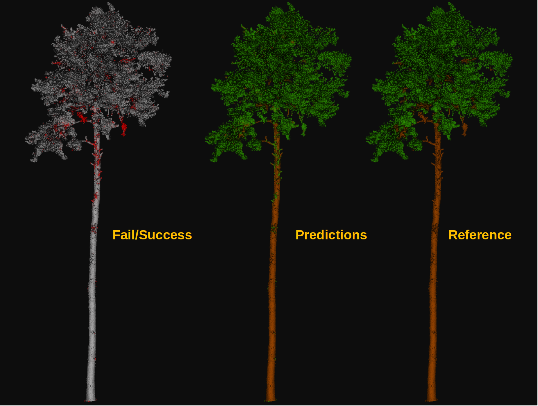
Visualization of the output obtained after computing a leaf-wood segmentation on a dataset containing a previously unseen tree. On the left, the red points represent misclassified points while the gray points represent successfully classified points. In the middle, the point-wise predicted labels (green for leaf, brown for wood). In the right, the point-wise reference labels.