Transformers

Transformers are components that apply a transformation on the point cloud. They can be divided into class transformers (ClassTransformer) that transform the classification and predictions of the point cloud, feature transformers (FeatureTransformer) that transform the features of the point cloud, and point transformers (PointTransformers) that compute an advanced transformation on the point cloud that involves different information (e.g., spatial coordinates to derive receptive fields that can be used to reduce or propagate both features and classes).

Transformers are typically use inside pipelines to apply transformations to the point cloud at the current pipeline’s state. Readers are strongly encouraged to read the Pipelines documentation before looking further into transformers.

Class transformers

Class reducer

The ClassReducer takes an original set of \(n_I\) input classes and returns \(n_O\) output classes, where \(n_O < n_I\). It can be applied to the reference classification only or also to the predictions. On top of that, it supports a text report on the distributions with the absolute and relative frequencies and a plot of the class distribution before and after the transformation. A ClassReducer can be defined inside a pipeline using the JSON below:

{
        "class_transformer": "ClassReducer",
        "on_predictions": false,
        "input_class_names": ["noclass", "ground", "vegetation", "cars", "trucks", "powerlines", "fences", "poles", "buildings"],
        "output_class_names": ["noclass", "ground", "vegetation", "buildings", "objects"],
        "class_groups": [["noclass"], ["ground"], ["vegetation"], ["buildings"], ["cars", "trucks", "powerlines", "fences", "poles"]],
        "report_path": "class_reduction.log",
        "plot_path": "class_reduction.svg"
}

The JSON above defines a ClassReducer that will replace the nine original classes into five reduced classes where many classes are grouped together as the "objects" class. Moreover, it will generate a text report in a file called class_reduction.log and a figure representing the class distribution in class_reduction.svg.

Arguments

– on_predictions

Whether to also reduce the predictions if any (True) or not (False). Note that setting on_predictions to True will only work if there are available predictions.

– input_class_names

A list with the names of the input classes.

– output_class_names

A list with the desired names for the output classes.

– class_groups

A list of lists such that the list i defines which classes will be considered to obtain the reduced class i. In other words, each sublist contains the strings representing the names of the input classes that must be mapped to the output class.

– report_path

Path where the text report on the class distributions must be written. If it is not given, then no report will be generated.

– plot_path

Path where the plot of the class distributions must be written. If it is not given, then no plot will be generated.

Output

The examples in this section come from applying a ClassReducer to the 5080_54435.laz point cloud of the DALES dataset .

An example of the plot representing how the classes are distributed before and after the ClassReducer is shown below.

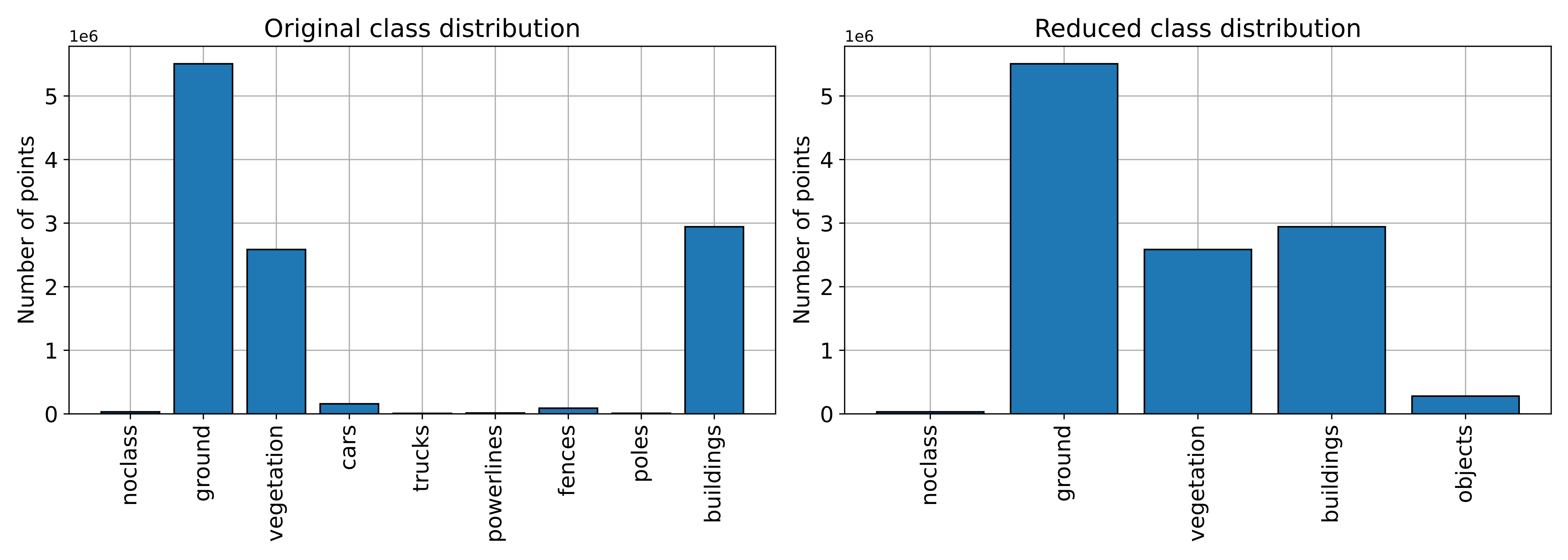
Visualization of the class distributions before and after the class reduction.

An example of how the classes represented on the point cloud look like before and after the ClassReducer is shown below.

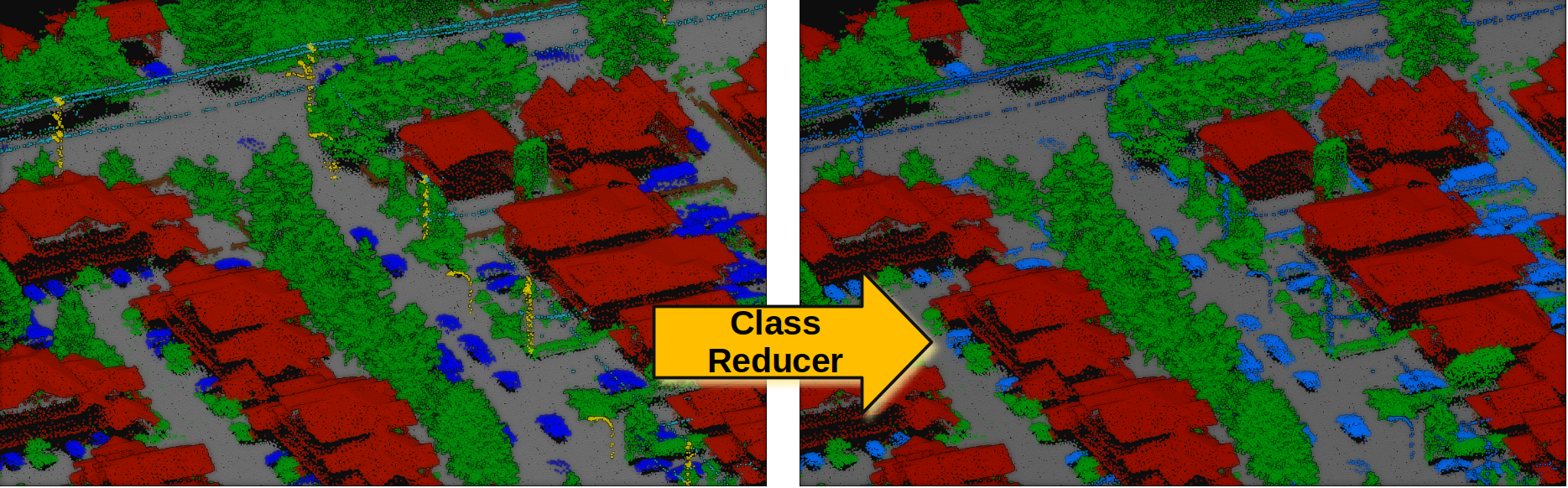
Visualization of the original (left) and reduced classification (right).

Class setter

The ClassSetter assigns the classes of a point cloud from any of its attributes. A ClassSetter can be defined inside a pipeline using the JSON below:

{
    "class_transformer": "ClassSetter",
    "fname": "Prediction"
}

The JSON above defines a ClassSetter that will assign the "Prediction" attribute as the point-wise classes of the point cloud.

Arguments

– fname

The name of the attribute that must be considered as the new classification of the point cloud.

Distance reclassifier

The DistanceReclassifier takes an original set of \(n_I\) input classes and returns \(n_O\) output classes. It can be applied to the reference classification or to the predictions. The transformation is based on relational filters, k-nearest neighbors neighborhoods, and point-wise distances involving the structure and feature spaces. It also supports a text report on the distributions with the absolute and relative frequencies and a plot of the class distribution before and after the transformation. A DistanceReclassifier can be defined inside a pipeline using the JSON below:

{
    "class_transformer": "DistanceReclassifier",
    "on_predictions": false,
    "input_class_names": ["ground", "vegetation", "building", "other"],
    "output_class_names": ["ground", "lowveg", "midveg", "highveg", "building", "other"],
    "reclassifications": [
      {
        "source_classes": ["vegetation"],
        "target_class": "highveg",
        "conditions": null,
        "distance_filters": null
      },
      {
        "source_classes": ["vegetation"],
        "target_class": "lowveg",
        "conditions": [
          {
            "value_name": "floor_dist",
            "condition_type": "less_than",
            "value_target": 0.5,
            "action": "preserve"
          }
        ],
        "distance_filters": null
      },
      {
        "source_classes": ["vegetation"],
        "target_class": "lowveg",
        "conditions": null,
        "distance_filters": [
          {
            "metric": "euclidean",
            "components": ["z"],
            "knn": {
              "coordinates": ["x", "y"],
              "max_distance": null,
              "k": 1,
              "source_classes": ["ground"]
            },
            "filter_type": "less_than",
            "filter_target": 1.0,
            "action": "preserve"
          }
        ]
      },
      {
        "source_classes": ["vegetation"],
        "target_class": "midveg",
        "conditions": null,
        "distance_filters": [
          {
            "metric": "euclidean",
            "components": ["z"],
            "knn": {
              "coordinates": ["x", "y"],
              "max_distance": null,
              "k": 1,
              "source_classes": ["ground"]
            },
            "filter_type": "inside",
            "filter_target": [1.0, 5.0],
            "action": "preserve"
          }
        ]
      }
    ],
    "report_path": "reclassification.log",
    "plot_path": "reclassification.svg",
    "nthreads": -1
}

The JSON above defines a DistanceReclassifier that will preserve the ground, building, and other classes while transforming the vegetation class into lowveg (low vegetation), midveg (mid vegetation), and highveg (high vegetation). In the process, it will generate a text report in a file called reclassification.log and a figure representing the class distributions in reclassification.svg.

Arguments

– on_predictions

Whether to also reduce the predictions if any (True) or not (False). Note that setting on_predictions to True will only work if there are available predictions.

– input_class_names

A list with the names of the input classes.

– output_class_names

A list with the desired names for the output/transformed classes.

– reclassifications

A list of dictionaries such that each dictionary specifies a class transform operation.

– source_classes

The names of the classes such that only points of these classes will be modified by the reclassification operation.

– target_class

The name of the target/output class to which those points that satisfy the conditions and distance-based filters will be assigned.

– conditions

A list of dictionaries such that each dictionary specifies a relational filter. See documentation about advanced input conditions .

– value_name

See documentation about advanced input conditions value name .

– condition_type

See documentation about advanced input condition type .

– value_target

See documentation about advanced input conditions value target .

– action

See documentation about advanced input conditions action .

– distance_filters

A list of dictionaries where each dictionary specifies a distance-based filter.

– metric

The distance metric to be computed for \(n\) components. It can be either "euclidean"

\[\operatorname{d}(\pmb{p}, \pmb{q}) = \sqrt{\sum_{j=1}^{n}{(p_j-q_j)^2}}\]

or "manhattan"

\[\operatorname{d}(\pmb{p}, \pmb{q}) = \sum_{j=1}^{n}{\left\lvert{p_j-q_j}\right\rvert} .\]

– components

A list with the names of the components defining the vectors whose distance will be computed. Supported components are "x", "y", and "z" for the corresponding coordinates from the structure space and also any feature name from the point cloud’s feature space.

– knn

The dictionary with the k-nearest neighbor neighborhood specification.

– coordinates

The coordinates defining the points for the neighborhood computations. For example, ["x", "y", "z"] implies typical 3D neighborhoods and ["x", "y"] implies typical 2D neighborhoods.

– max_distance

The max distance that any neighbor must satisfy. Points further away than this distance will be excluded from the neighborhood.

– k

The number of \(k\)-nearest neighbors.

– source_classes

Neighborhoods will only contain points belonging to the given source classes. If None, then all points will be considered as neighbors, no matter their class.

– filter_type

Like the advanced input condition type specification but also supports "inside" (\(x \in [a, b] \subset \mathbb{R}\)).

– filter_target

See documentation about advanced input conditions value target .

– action

See documentation about advanced input conditinos action .

– report_path

Path where the text report on the class distributions must be written. If it is not given, then no report will be generated.

– plot_path

Path where the plot of the class distributions must be written. If it is not given, then no plot will be generated.

– nthreads

The number of threads for the parallel computations. Note that using -1 means as many threads as available cores.

Output

The examples in this section come from applying a DistanceReclassifier to the PNOA_2015_GAL-W_478-4766_ORT-CLA-COL point cloud of the PNOA-II dataset .

The figure below is the plot representing how the classes are distributed before and after the DistanceReclassfier.

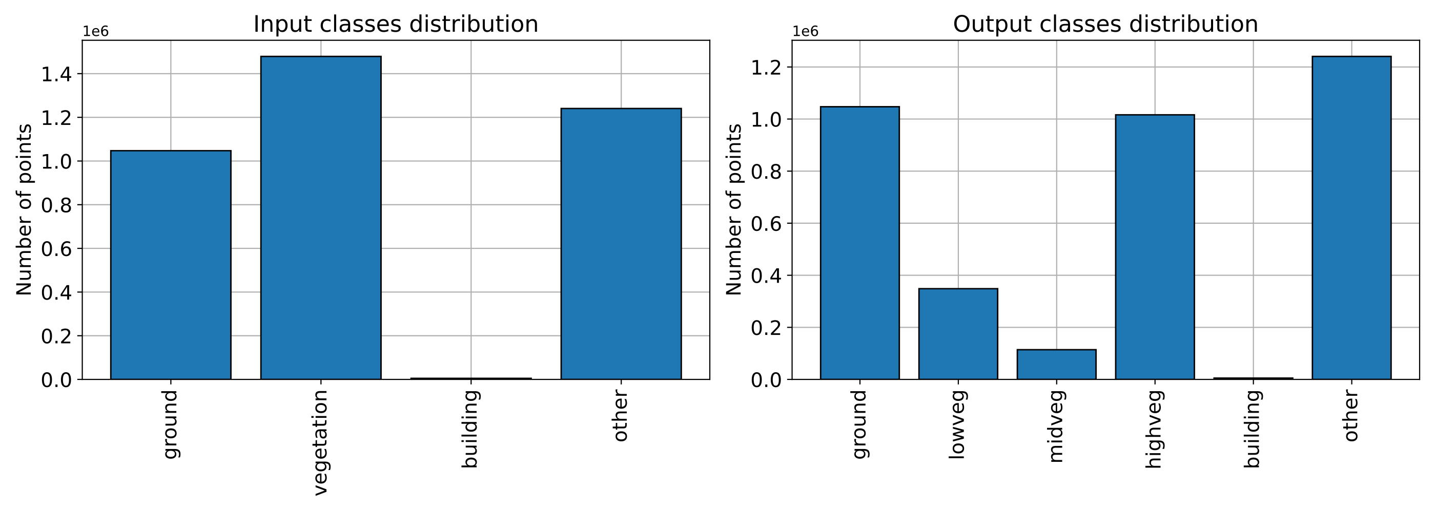
Visualization of the class distributions before and after the distance-based reclassification.

The figure below represents the vegetation reclassified by heights following the specifications from the JSON above (note that the floor distance was computed using the height features miner ++).

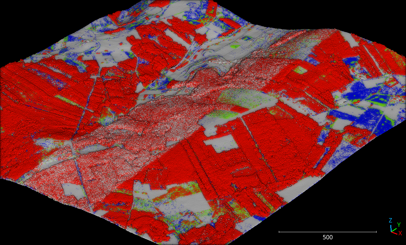
Visualization of the reclassified point cloud. Non-vegetation classes are colored white, low vegetation points are blue, mid vegetation ones are green, and high vegetation is red.

Feature transformers

Minmax normalizer

The MinmaxNormalizer maps the specified features so they are inside the \([a, b]\) interval. It can be configured to clip values outside the interval or not. If so, values below \(a\) will be replaced by \(a\) while values above \(b\) will be replaced by \(b\). A MinmaxNormalizer can be defined inside a pipeline using the JSON below:

{
    "feature_transformer": "MinmaxNormalizer",
    "fnames": ["AUTO"],
    "target_range": [0, 1],
    "clip": true,
    "report_path": "minmax_normalization.log"
}

The JSON above defines a MinmaxNormalizer that will map the features to be inside the \([0, 1]\) interval. If this transformer is later applied to different data, it will make sure that there is not value less than zero or greater than one. On top of that, a report about the normalization will be written to the minmax_normalization.log text file.

Arguments

– fnames

The names of the features to be normalized. If "AUTO", the features considered by the last component that operated over the features will be used.

– target_range

The interval to normalize the features.

– clip

When a minmax normalizer has been fit to a dataset, it will find the min and max values to compute the normalization. It can be that the normalizer is then applied to other dataset with different min and max. Under those circumstances, values below \(a\) or above \(b\) might appear. When clip is set to true, this values will be replaced by either \(a\) or \(b\) so the normalizer never yields values outside the \([a, b]\) interval.

– minmax

An optional list of pairs (e.g., list of lists, where each sublist has exactly two elements). When given, each i-th element is a pair where the first component gives the min for the i-th feature and the second one gives the max.

– frenames

An optional list of names. When given, the normalized features will use these names instead of the original ones given by fnames.

– report_path

When given, a text report will be exported to the file pointed by the path.

– update_and_preserve

When true, the features that were not transformed by minmax normalization will be kept in the point cloud with the normalized features. When false, the values of non-transformed features might be missing.

Output

A transformed point cloud is generated such that its features are normalized to a [0, 1] interval. The min, the max, and the range are exported through the logging system (see below for an example corresponding to the minmax normalization of some geometric features).

FEATURE	MIN	MAX	RANGE
linearity_r0.05	0.00028	1.00000	0.99972
planarity_r0.05	0.00000	0.97660	0.97660
surface_variation_r0.05	0.00000	0.32316	0.32316
eigenentropy_r0.05	0.00006	0.01507	0.01501
omnivariance_r0.05	0.00000	0.00060	0.00060
verticality_r0.05	0.00000	1.00000	1.00000
anisotropy_r0.05	0.06250	1.00000	0.93750
linearity_r0.1	0.00070	1.00000	0.99930
planarity_r0.1	0.00000	0.95717	0.95717
surface_variation_r0.1	0.00000	0.32569	0.32569
eigenentropy_r0.1	0.00028	0.04501	0.04473
omnivariance_r0.1	0.00000	0.00241	0.00241
verticality_r0.1	0.00000	1.00000	1.00000
anisotropy_r0.1	0.05643	1.00000	0.94357

Standardizer

The Stantardizer maps the specified features so they are transformed to have mean zero \(\mu = 0\) and standard deviation one \(\sigma = 1\). Alternatively, it is possible to only center (mean zero) or scale (standard deviation one) the data. A Standardizer can be defined inside a pipeline using the JSON below:

{
    "feature_transformer": "Standardizer",
    "fnames": ["AUTO"],
    "center": true,
    "scale": true,
    "report_path": "standardization.log"
}

The JSON above defines a Standardizer that centers and scales the data. Besides, it will export a text report with the feature-wise means and variances to the standardization.log file.

Arguments

– fnames

The names of the features to be standardized. If "AUTO", the features considered by the last component that operated over the features will be used.

– center

Whether to subtract the mean (true) or not (false).

– scale

Whether to divide by the standard deviation (true) or not (false).

– report_path

When given, a text report will be exported to the file pointed by the path.

– update_and_preserve

When true, the features that were not transformed through normalization (i.e., standardization) will be kept in the point cloud with the normalized features. When false, the values of non-transformed features might be missing.

Output

A transformed point cloud is generated such that its features are standardized. The mean and standard deviation are exported through the logging system (see below for an example corresponding to the standardization of some geometric features).

FEATURE	MEAN	STDEV.
linearity_r0.05	0.47259	0.24131
planarity_r0.05	0.32929	0.22213
surface_variation_r0.05	0.10697	0.06362
eigenentropy_r0.05	0.00781	0.00184
omnivariance_r0.05	0.00025	0.00010
verticality_r0.05	0.55554	0.30274
anisotropy_r0.05	0.80188	0.14316
linearity_r0.1	0.49389	0.24075
planarity_r0.1	0.29196	0.21008
surface_variation_r0.1	0.11583	0.06376
eigenentropy_r0.1	0.02512	0.00533
omnivariance_r0.1	0.00100	0.00035
verticality_r0.1	0.57260	0.30121
anisotropy_r0.1	0.78585	0.14570

Variance selector

The variance selection is a simple strategy that consists of discarding all those features which variance lies below a given threshold. While simple, the VarianceSelector has a great strength and that is it can be computed without known classes because it is based only on the variance. A VarianceSelector can be defined inside a pipeline using the JSON below:

{
    "feature_transformer": "VarianceSelector",
    "fnames": ["AUTO"],
    "variance_threshold": 0.01,
    "report_path": "variance_selection.log"
}

The JSON above defines a VarianceSelector that removes all features which variance is below \(10^{-2}\). After that, it will export a text report describing the process to the variance_selection.log file.

Arguments

– fnames

The names of the features to be transformed. If "AUTO", the features considered by the last component that operated over the features will be used.

– variance_threshold

Features which variance is below this threshold will be discarded.

– report_path

When given, a text report will be exported to the file pointed by the path.

Output

A transformed point cloud is generated considering only the features that passed the variance threshold. On top of that, the feature-wise variances are exported through the logging system. The selected features are also explicitly listed (see below for an example corresponding to a variance selection on some geometric features).

FEATURE	VARIANCE
omnivariance_r0.05	0.000
omnivariance_r0.1	0.000
eigenentropy_r0.05	0.000
eigenentropy_r0.1	0.000
surface_variation_r0.05	0.004
surface_variation_r0.1	0.005
anisotropy_r0.05	0.020
anisotropy_r0.1	0.022
linearity_r0.1	0.051
linearity_r0.05	0.056
planarity_r0.1	0.066
planarity_r0.05	0.075
verticality_r0.05	0.092
verticality_r0.1	0.097

SELECTED FEATURES
linearity_r0.05
planarity_r0.05
verticality_r0.05
anisotropy_r0.05
linearity_r0.1
planarity_r0.1
verticality_r0.1
anisotropy_r0.1

K-Best selector

The KBestSelector computes the feature-wise ANOVA F-values and use them to sort the features. Then, only the \(K\) best features, i.e., those with highest F-values, will be preserved. A KBestSelector can be defined inside a pipeline using the JSON below:

{
    "feature_transformer": "KBestSelector",
    "fnames": ["AUTO"],
    "type": "classification",
    "k": 2,
    "report_path": "kbest_selection.log"
}

The JSON above defines a KBestSelector that computes the ANOVA F-Values assuming a classification task. Then, it discards all features but the two with the highest values. Finally, it writes a text report with the feature-wise F-Values and the associated p-value for each test to the file kbest_selection.log

Arguments

– fnames

The names of the features to be transformed. If "AUTO", the features considered by the last component that operated over the features will be used.

– type

Specify which type of task is going to be computed. Either, "regression" or "classification". The F-Values computation will be carried out to be adequate for one of those tasks. For regression tasks the target variable is expected to be numerical, while for classification tasks it is expected to be categorical.

– k

How many top-features must be preserved.

– report_path

When given, a text report will be exported to the file pointed by the path.

Output

A transformed point cloud is generated considering only the K-best features according to the F-values. Moreover, the feature-wise F-Values and their associated p-value are exported through the logging system. The selected features are also explicitly listed (see below for an example corresponding to a K-best selection on some geometric features).

FEATURE	F-VALUE	P-VALUE
eigenentropy_r0.1	811.946	0.000
omnivariance_r0.05	1050.085	0.000
linearity_r0.05	2290.284	0.000
planarity_r0.1	4795.994	0.000
linearity_r0.1	16100.821	0.000
eigenentropy_r0.05	16307.772	0.000
anisotropy_r0.05	17643.102	0.000
surface_variation_r0.05	18972.138	0.000
planarity_r0.05	19226.943	0.000
omnivariance_r0.1	20649.736	0.000
verticality_r0.05	90577.769	0.000
verticality_r0.1	106840.172	0.000
anisotropy_r0.1	116002.960	0.000
surface_variation_r0.1	122409.281	0.000

SELECTED FEATURES
surface_variation_r0.1
anisotropy_r0.1

Percentile selector

The PercentileSelector computes the ANOVA F-Values and use them to sort the features. Then, only a given percentage of the features are preserved. More concretely, the given percentage of the features with the highest F-Values will be preserved. A PercentileSelector can be defined inside a pipeline using the JSON below:

{
    "feature_transformer": "PercentileSelector",
    "fnames": ["AUTO"],
    "type": "classification",
    "percentile": 20,
    "report_path": "percentile_selection.log"
}

The JSON above defines a PercentileSelector that computes the ANOVA F-Values assuming a classification task. Then, it preserves the \(20\%\) of the features with the highest F-Values. Finally, it writes a text report with the feature-wise F-Values and the associated p-value for each test to the file percentile_selection.log.

Arguments

– fnames

The names of the features to be transformed. If "AUTO", the features considered by the last component that operated over the features will be used.

– type

Specify which type of task is going to be computed. Either, "regression" or "classification". The F-Values computation will be carried out to be adequate for one of those tasks. For regression tasks the target variable is expected to be numerical, while for classification tasks it is expected to be categorical.

– percentile

An integer from \(0\) to \(100\) that specifies the percentage of top-features to preserve.

– report_path

When given, a text report will be exported to the file pointed by the path.

Output

A transformed point cloud is generated considering only the requested percentage of best features according to the F-values. Moreover, the feature-wise F-Values and their p-value are exported through the logging system. The selected features are also explicitly listed (see below for an example corresponding to a percentile selection on some geometric features).

FEATURE	F-VALUE	P-VALUE
eigenentropy_r0.1	811.946	0.000
omnivariance_r0.05	1050.085	0.000
linearity_r0.05	2290.284	0.000
planarity_r0.1	4795.994	0.000
linearity_r0.1	16100.821	0.000
eigenentropy_r0.05	16307.772	0.000
anisotropy_r0.05	17643.102	0.000
surface_variation_r0.05	18972.138	0.000
planarity_r0.05	19226.943	0.000
omnivariance_r0.1	20649.736	0.000
verticality_r0.05	90577.769	0.000
verticality_r0.1	106840.172	0.000
anisotropy_r0.1	116002.960	0.000
surface_variation_r0.1	122409.281	0.000

SELECTED FEATURES
surface_variation_r0.1
verticality_r0.1
anisotropy_r0.1

Explicit selector

The ExplicitSelector preserves or discards the requested features, thus effectively updating the point cloud in the pipeline’s state (see SimplePipelineState). This feature transformation can be especially useful to release memory resources by discarding features that are not going to be used by other components later on. A ExplicitSelector can be defined inside a pipeline using the JSON below:

{
    "feature_transformer": "ExplicitSelector",
    "fnames": [
        "floor_distance_r50_0_sep0_35"
        "scan_angle_rank_mean_r5_0",
        "verticality_r25_0"
    ],
    "preserve": true
}

The JSON above defines a ExplicitSelector that preserves the floor distance, mean scan angle, and verticality features. In doing so, all the other features are discarded. After calling this selector, only the preserved features will be available through the pipeline’s state.

Arguments

– fnames

The names of the features to be either preserved or discarded.

– preserve

The boolean flag that governs whether the given features must be preserved (true) or discarded (false).

Output

A transformed point cloud is generated considering only the preserved features.

PCA transformer

The PCATransformer can be used to compute a dimensionality reduction of the feature space. Let \(\pmb{F} \in \mathbb{R}^{m \times n_f}\) be a matrix of features such that each row \(\pmb{f}_{i} \in \mathbb{R}^{n_f}\) represents the \(n_f\) features for a given point \(i\). After applying the PCA transformer a new matrix of features will be obtained \(\pmb{Y} \in \mathbb{R}^{m \times n_y}\) such that \(n_y \leq n_f\). This dimensionality reduction can help reducing the number of input features for a machine learning model, and consequently reducing the execution time.

To understand this transformation, simply note the singular value decomposition of \(\pmb{F} = \pmb{U} \pmb{\Sigma} \pmb{V}^\intercal\). The singular vectors in \(\pmb{V}^\intercal\) can be ordered in descendant order from higher to lower singular value, where singular values are given by the diagonal of \(\pmb{\Sigma}\). Alternatively, the basis matrix defined by the singular vectors can be approximated with the eigenvectors of the centered covariance matrix. From now on, no matter how it was computed, we will call this basis matrix \(\pmb{B}\). We also assume that we always have enough linearly independent features for the analysis to be feasible.

When all the basis vectors are considered, it will be that \(\pmb{B} \in \mathbb{R}^{n_f \times n_f}\), i.e., \(n_y=n_f\). In this case we are expressing potentially correlated features in a new basis where each feature aims to be orthogonal w.r.t. the others (principal components). When \(\pmb{B} \in \mathbb{R}^{n_f \times n_y}\) for \(n_y<n_f\), and the basis contains the singular vectors corresponding to the higher singular values , we are reducing the dimensionality using a subset of the principal components. This dimensionality reduction transformation will preserve as much variance as possible in the data while using less orthogonal features.

A PCATransformer can be defined inside a pipeline using the JSON below:

{
    "feature_transformer": "PCATransformer",
    "fnames": ["AUTO"],
    "out_dim": 0.99,
    "whiten": false,
    "random_seed": null,
    "report_path": "pca_projection.log",
    "plot_path": "pca_projection.svg",
    "update_and_preserve": false
}

The JSON above defines a PCATransformer that considers as many principal components as necessary to explain the \(99\%\) of the variance. On top of that, it will export a text report with the aggregated contribution to the explained variance of the considered principal components (ordered from most significant to less significant) to a file named pca_projection.log. Finally, it will also export a plot representing the explained variance ratio as a function of the output dimensionality to a file named pca_projection.svg.

Arguments

– fnames

The names of the features to be transformed. If "AUTO", the features considered by the last component that operated over the features will be used.

– out_dim

The ratio of preserved features governing the output dimensionality. It is a value in \((0, 1]\) where 1 implies \(n_y=n_f\) and less than one governs how small is \(n_y\) with respect to \(n_f\).

– whiten

When true, the singular vectors will be scaled by the square root of the number of points and divided by the corresponding singular value. Consequently, the output will consists of features with unit variance. When false, nothing will be done.

– random_seed

Can be used to specify a seed (as an integer) for reproducibility purposes when using randomized solvers for the computations.

– report_path

When given, a text report will be exported to the file pointed by the path.

– plot_path

When given, a plot representing the explained variance ratio as a function of the number of considered principal components will be exported to the file pointed by the path.

– update_and_preserve

When true, the features transformed through PCA will be discarded, but those that were not considered will be kept in the point cloud together with the PCA-based features. When false (by default), the point cloud will only contain the PCA-based features.

Output

A transformed point cloud is generated with the new features obtained by the PCATransformer. Moreover, the explained variances will be exported through the logging system.

FEATURE	EXPLAINED VAR. (%)
PCA_8	2.9685
PCA_7	3.9065
PCA_6	5.5666
PCA_5	6.9705
PCA_4	9.0035
PCA_3	12.0645
PCA_2	22.4750
PCA_1	36.2546

Furthermore, if requested a plot will be exported to a file. This plot describes the explained variance ratio as a function of the number of output features (output dimensionality). An example can be see below where the PCATransformer was used to reduce 14 features into 8 features that explain at least a \(99\%\) of the variance.

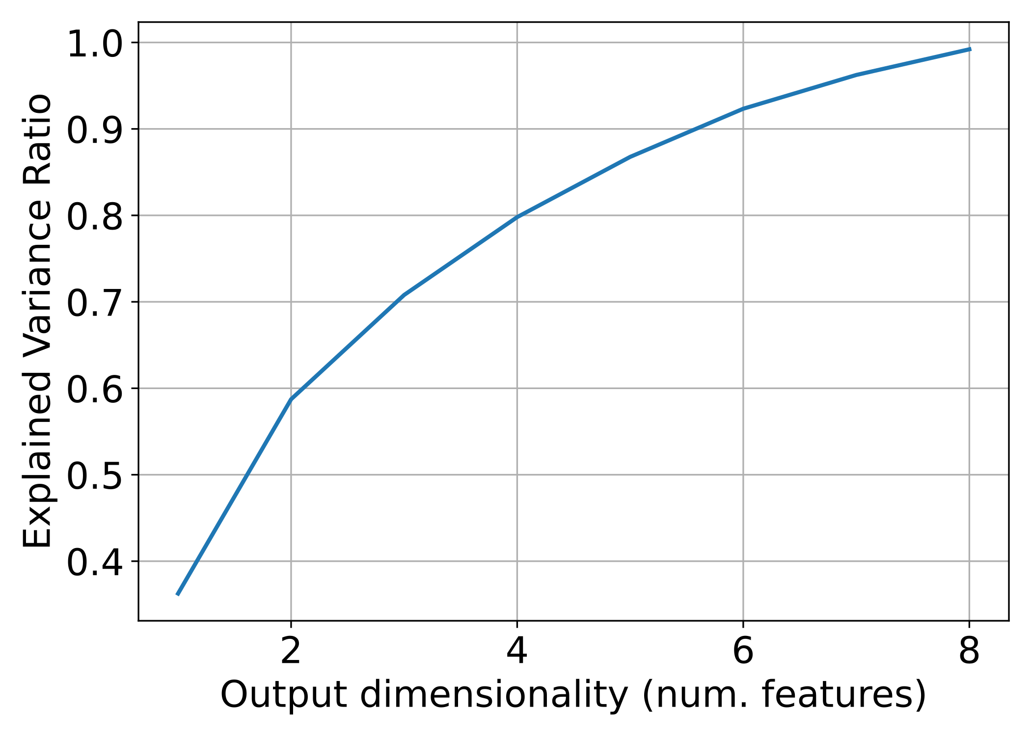
The relationship between the PCA-derived features and the aggregated explained variance ratio.

Finally, the image below represents how three different features were reduced to a single one using PCA. The output point cloud can be exported using a Writer component (see Writer documentation).

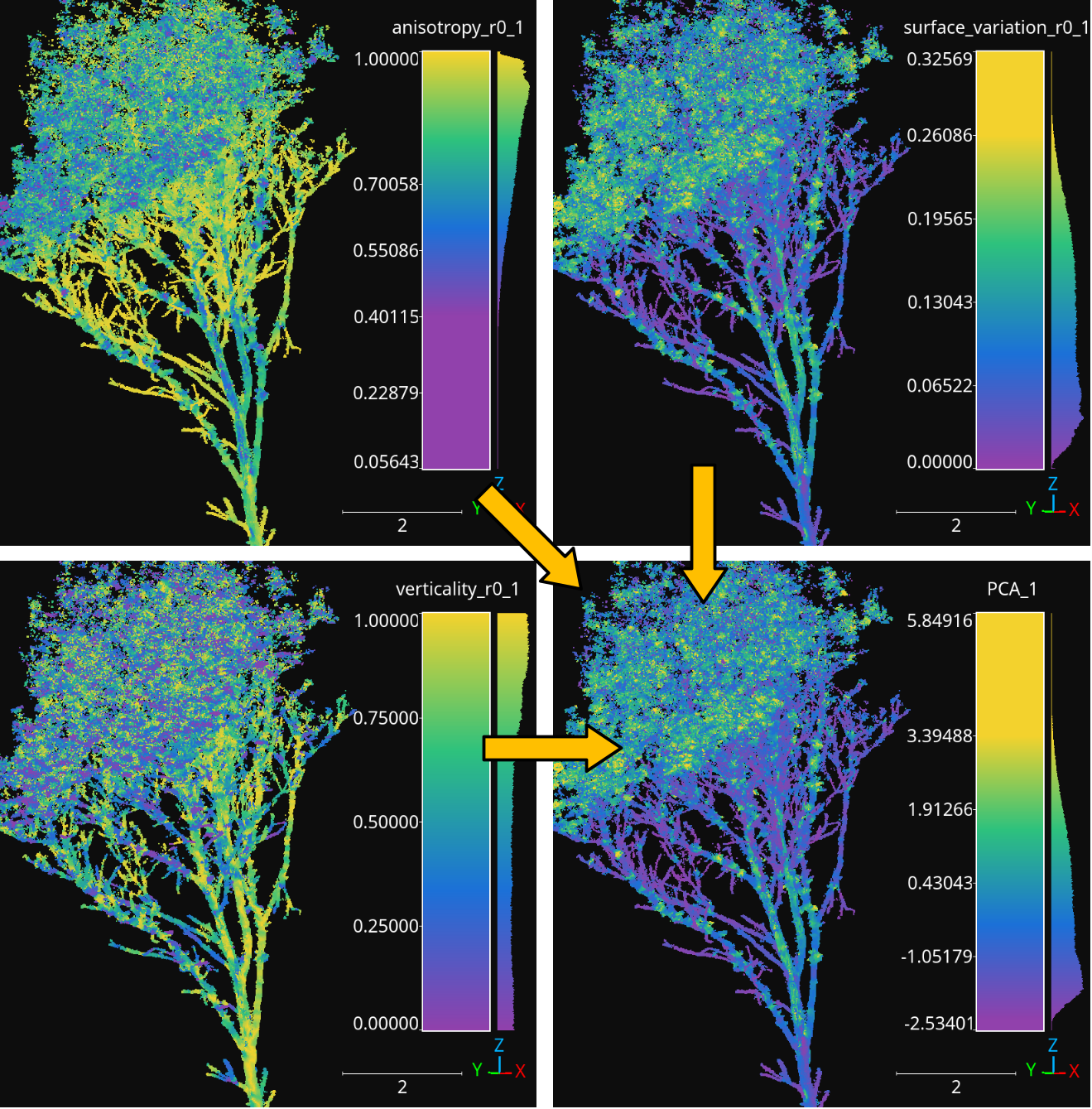
The anisotropy, surface variation, and verticality computed for spherical neighborhoods with \(10\,\mathrm{cm}\) radius reduced to a single feature through PCA.

Point transformers

Some point transformers like ReceptiveField or DataAugmentor and their derived classes (e.g., ReceptiveFieldFPS, ReceptiveFieldGS, ReceptiveFieldHierarchicalFPS, SimpleDataAugmentor )are used in the context of deep learning models. Thus, they are not available as independent components for pipelines. Other point transformers, typically those that extend PointTransformer can be used as components in pipelines and are detailed here.

Point cloud sampler

The PointCloudSampler generates a new point cloud by sampling from the current one (i.e., the point cloud in the pipeline’s state, see documentation on pipelines). A PointCloudSampler can be defined inside a pipeline using the JSON below:

{
    "point_transformer": "PointCloudSampler",
    "neighborhood_sampling": {
        "support_conditions": [
            {
                "value_name": "HighCA_rel",
                "condition_type": "greater_than_or_equal_to",
                "value_target": 0.667,
                "action": "preserve"
            }
        ],
        "support_min_distance": 1.25,
        "support_strategy": "fps",
        "support_strategy_num_points": 100000,
        "support_strategy_fast": true,
        "support_chunk_size": 50000,
        "center_on_pcloud": false,
        "neighborhood": {
            "type": "sphere",
            "radius": 2.5,
            "separation_factor": 0
        },
        "neighborhoods_per_iter": 10000,
        "nthreads": -1
    }
}

The JSON above defines a PointCloudSampler that will generate a point cloud considering spherical neighborhoods with radius \(2.5\,\mathrm{m}\) centered on those points in the current point cloud with a relative frequency of high class ambiguity neighbors greater than or equal to \(0.667\). A point is said to have a high class ambiguity if it is greater than or equal to \(0.667\). When sampling, all the center points that are close to each other in less than \(1.25\,\mathrm{m}\).

Arguments

– fnames

The names of the features that must be included in the sampled point cloud. If null, then all the available features will be included.

– neighborhood_sampling

When null, no neighborhood sampling will be applied. If given, it must be a key-word specification of the desired neighborhood sampling strategy, as described below:

– support_conditions

A list with the conditions that must be satisfied by any center point whose neighborhood could be included in the generated point cloud (provided it satisfies the other criteria). The specification for each conditions is similar to the one described in the conditions for advanced input documentation.

– support_min_distance

When more there are many center points that are close to each other in less than this distance, only one will be considered.

– support_strategy

If the support points are not calculated with a null separation factor, then the support strategy will be used to select the initial candidates. See the receptive fields documentation for further details because the specification works in the same way.

– support_strategy_num_points

If the support points are not calculated with a null separation factor, and the "fps" support strategy is used, then this number of points will govern the number of initially selected candidates. See the receptive fields documentation for further details because the specification works in the same way.

– support_strategy_fast

If the support points are not calculated with a null separation factor, fast heuristics can be applied to speedup the computations. See FPS receptive field documentation for further details.

– support_chunk_size

When given and distinct than zero, it will define the chunk size. The chunk size will be used to group certain tasks into chunks with a max size to prevent memory exhaustion.

– center_on_pcloud

When true the neighborhoods will be centered on a point from the input point cloud. Typically by finding the nearest neighbor of a support point in the input point cloud. In general, it is recommended to set it to false for most use cases of the PointCloudSampler.

– neighborhoods_per_iter

When doing multiple iterations to compute the neighborhoods, the overlapping might yield many repeated points. However, there is no need to store repeated elements in memory (which can be prohibitive). When the number of neighborhoods per iter is set to be greater than zero, only this number of neighborhoods will be computed at once, thus controlling the required memory.

– nthreads

The number of threads involved in parallel computations, if any.

– neighborhood

The definition of the neighborhood. See the FPS neighborhood specification for further details because it follows the same format.

– type

Supported neighborhood types are: "sphere", "cylinder", "rectangular3d", and "rectangular2d".

– radius

A decimal number goverening the size of the neighborhood.

– separation_factor

A decimal number governing the separation between neighborhoods. It it recommended to set it to zero so the custom support extraction strategy of the PointCloudSampler is used.

Output

A point cloud is generated by sampling spherical neighborhoods from high class ambiguity regions in the original point cloud. The class ambiguity has been measured for a KPConv-like neural network model. The point cloud is taken from the Architectural Cultural Heritage (ArCH) dataset .

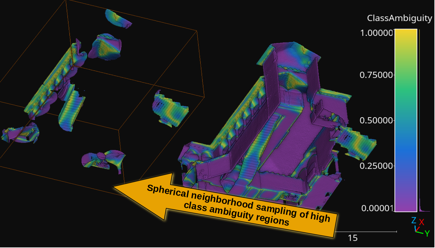
The spherical neighborhoods sampled from high class ambiguity regions (those inside the orange bounding box). The points are colored by class ambiguity.

Simple structure smoother++

The SimpleStructureSmootherPP generates a new point cloud by smoothing the coordinates of each point considering its local neighborhood. A SimpleStructureSmootherPP can be defined inside a pipeline using the JSON below:

{
  "point_transformer": "SimpleStructureSmootherPP",
  "neighborhood": {
    "type": "sphere",
    "radius": 20,
    "k": 1024
  },
  "strategy": {
    "type": "idw",
    "parameter": 2,
    "min_distance": 4
  },
  "correction": {
    "K": 0,
    "sigma": 3.14159265358979323846264338327950288419716939937510
  },
  "nthreads": -1
}

The JSON above defines a SimpleStructureSmoother applied on spherical neighborhoods with \(20\;\mathrm{mm}\) radius using inverse distance weighting with \(p=2\) and \(\epsilon=4\). It does not use Fibonacci orthodromic correction at all.

Arguments

– neighborhood

The definition of the neighborhood.

– type

The type of neighborhood. It can be either "knn" (3D k-nearest neighbors), "knn2d" (2D k-nearest neighbors considering the \((x, y)\) coordinates only), "sphere" (spherical neighborhood), and "cylinder" (cylindrical neighborhood).

– radius

The radius for the sphere or the disk of the cylinder.

– k

The number of k-nearest neighbors.

– strategy

The specification of the smoothing strategy.

– type

The smoothing strategy. It can be either "mean", "idw" (Inverse Distance Weighting), or "rbf" (Radial Basis Function).

– parameter

The \(p \in \mathbb{R}\) parameter for the IDW exponent or the Gaussian RBF bandwith.

– min_distance

The \(\epsilon \in \mathbb{R}\) parameter governing the min distance for IDW smoothing. Distances smaller than this will be replaced.

– correction

The configuration of the Fibonacci orthodromic correction.

– K

The number of pionts in the spherical Fibonacci support. The greater the better but it will lead to higher execution times (i.e., it increases the computational cost).

– sigma

The hard cut threshold for the Fibonacci orthodromic correction between a point in a centered neighborhood \(\pmb{x}_{j*} \in \mathbb{R}^{3}\) and a point from the Fibonacci support \(\pmb{q}_{k*} \in \mathbb{R}^{3}\).

\[\omega(\pmb{x}_{j*}, \pmb{q}_{k*}) = \max \left\{ 0, \sigma - \arccos\left(\dfrac{ \langle\pmb{x}_{j*}, \pmb{q}_{k*}\rangle }{ \lVert\pmb{x}_{j*}\rVert } \right) \right\}\]

– nthreads

The number of threads to be used for parallel computations (-1 means as many threads as available cores).

Output Smoother versions of a point cloud using the JSON above with different parameters. The input data comes from the Head and Neck Organ-at-Risk CT Segmentation Dataset (HaN-Seg) dataset.

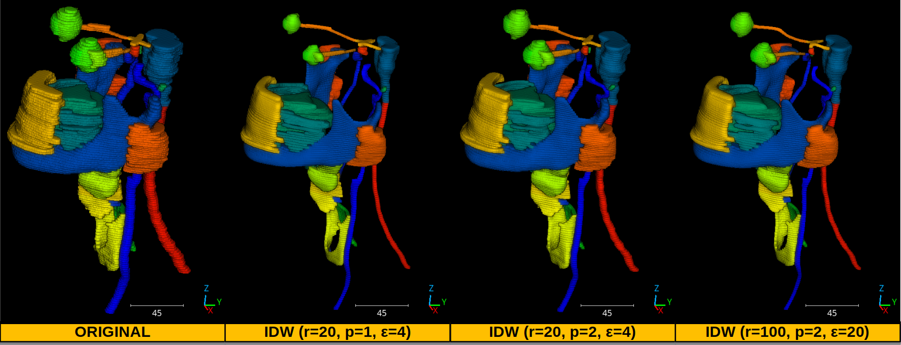
The smoothed versions of a medical 3D point cloud representing the head and neck regions. Each color represents a distinct organ.