Evaluators

Evaluators are components that can be used to evaluate the data, the model, or the predictions. The evaluations are typically represented through text reports, point clouds, and plots. An Evaluator component is typically used inside pipelines to assess the performance of a machine learning model or to understand the insights of a neural network. Readers should be familiar with pipelines to understand how to include evaluators in their workflows.

Classification evaluator

The ClassificationEvaluator assumes there is a labeled point cloud and that some predictions have been computed for that point cloud. It will consider the predictions and reference labels at the current pipeline’s state and will evaluate them in different ways. A ClassificationEvaluator can be defined inside a pipeline using the JSON below:

{
    "eval": "ClassificationEvaluator",
    "class_names": ["Ground", "Vegetation", "Building", "Urban furniture", "Vehicle"],
    "metrics": ["OA", "P", "R", "F1", "IoU", "wP", "wR", "wF1", "wIoU", "MCC", "Kappa"],
    "class_metrics": ["P", "R", "F1", "IoU"],
    "report_path": "*report/global_eval.log",
    "class_report_path": "*report/class_eval.log",
    "confusion_matrix_report_path" : "confusion_matrix.log",
    "confusion_matrix_plot_path" : "confusion_matrix.svg",
    "confusion_matrix_normalization_strategy": null,
    "class_distribution_report_path": "class_distribution.log",
    "class_distribution_plot_path": "class_distribution.svg",
    "nthreads": 1
}

The JSON above defines a ClassificationEvaluator that will consider many metrics, from the overall accuracy to the Cohen’s kappa score, to evaluate the predicted point clouds. Some metrics will also be considered to compute class-wise scores. On top of that, the confusion matrix and the distribution of the points among the classes will be analyzed. All the evaluations can be exported as a report, typically a text file containing the data or a plot for quick visualization.

Arguments

– class_names

A list with the names for the classes. These names will be used to represent the classes in the plots and the reports.

– metrics

The metrics to evaluate the classification. Supported class metrics are:

• "OA" Overall accuracy.

• "P" Precision.

• "R" Recall.

• "F1" F1 score (harmonic mean of precision and recall).

• "IoU" Intersection over union (also known as Jaccard index).

• "wP" Weighted precision (weights by the number of true instances for each class).

• "wR" Weighted recall (weights by the number of true instances for each class).

• "wF1" Weighted F1 score (weights by the number of true instances for each class).

• "wIoU" Weighted intersection over union (weights by the number of true instances for each class).

• "MCC" Matthews correlation coefficient.

• "Kappa" Cohen’s kappa score.

– class_metrics

The metrics to evaluate the classification in a class-wise way. Supported class metrics are:

• "P" Precision.

• "R" Recall.

• "F1" F1 score (harmonic mean of precision and recall).

• "IoU" Intersection over union (also known as Jaccard index).

– ignore_classes

Optional list of classes to be ignored when computing the evaluation metrics. Any point whose label matches a class in this list will be excluded. The classes must be given as a list of strings that matches those from class_names, i.e., ignore_classes \(\subseteq\) class_names.

– ignore_predictions

Whether to also ignore the classes in the predictions (true) or not (false, default). Note that it is strongly recommended to avoid ignoring the predictions, as it can lead to wrong interpretations of the model performance. Yet, it can be useful in some circumstances.

– report_path

Path to write the evaluation of the classification to a text file.

– class_report_path

Path to write the class-wise evaluation of the classification to a text file.

– confusion_matrix_report_path

Path to write the confusion matrix to a text file.

– confusion_matrix_plot_path

Path to write the plot representing a confusion matrix to a file.

– confusion_matrix_normalization_strategy

The strategy to normalize the confusion matrix (when plotting it), if any. It can be either "row" to apply a row-wise normalization (i.e., by references, recall), "col" to apply a column-wise normalization (i.e., by predictions, precision), or "full" to normalize considering the total number of samples. When not given (i.e., null), no normalization will be applied.

– class_distribution_report_path

Path to write the class distribution report to a text file.

– class_distribution_plot_path

Path to write the plot representing the class distribution to a text file.

– nthreads

The number of threads to use for the parallel computation of evaluation metrics. At most one thread per requested metric can be used. If set to -1 then as many threads as available cores will be used.

Output

The output is illustrated considering the March 2018 point clouds from the Hessigheim dataset to compute the classification’s evaluation.

The table below represents the confusion matrix exported as a CSV report. The rows represent the true labels, while the columns represent the predictions.

Ground	Vegetation	Building	Urban furniture	Vehicle
7117968	48936	246357	121840	9140
52931	1992443	215502	295401	3853
111624	42669	3499547	67170	215
72761	21997	199058	158505	3068
42451	8250	64580	29340	38642

The image below represents the confusion matrix as a figure. The information in the image is the same than the one in the table but in a different format.

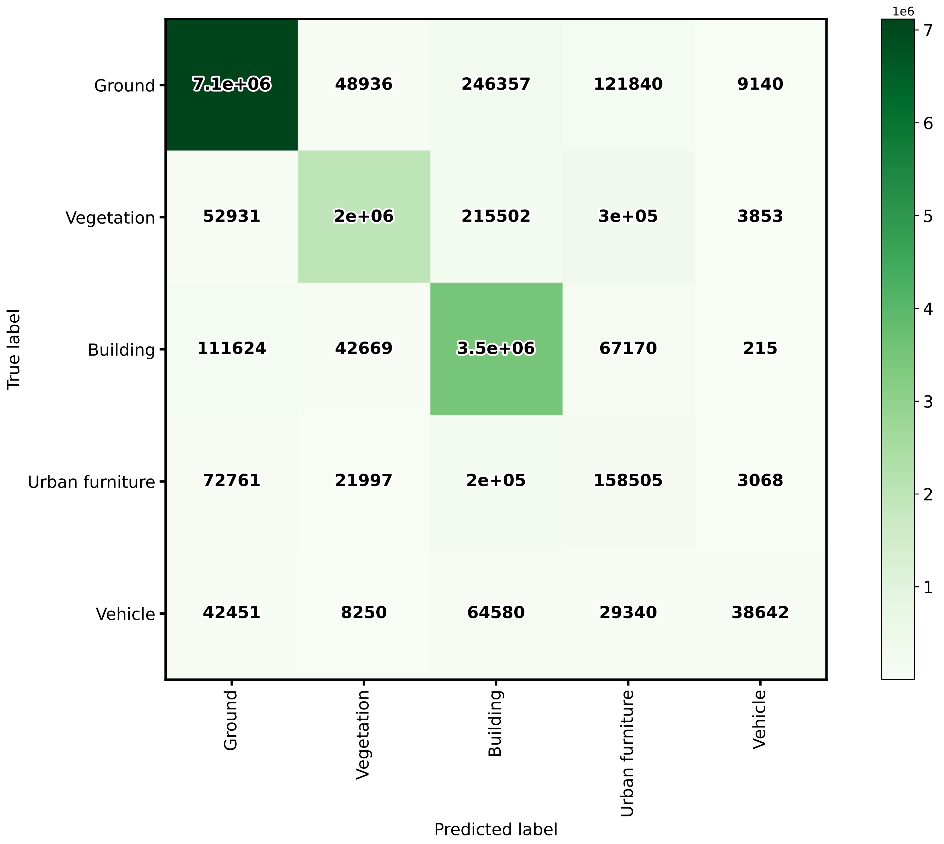
The confusion matrix exported by the classification evaluator.

Advanced classification evaluator

The AdvancedClassificationEvaluator uses the ClassificationEvaluator many times (see documentation), one per node in the analysis domain. It can be defined inside a pipeline using the JSON below:

{
    "eval": "AdvancedClassificationEvaluator",
    "class_names": ["vegetation", "other"],
    "metrics": ["OA", "P", "R", "F1", "IoU", "wP", "wR", "wF1", "wIoU", "MCC", "Kappa"],
    "class_metrics": ["P", "R", "F1", "IoU"],
    "report_path": "*report/global_eval.log",
    "plot_path": "*report/global_plot.svg",
    "class_report_path": "*report/class_eval.log",
    "class_plot_path": "*report/class_eval.svg",
    "confusion_matrix_report_path" : "*report/confusion_matrix.log",
    "confusion_matrix_plot_path" : "*report/confusion_matrix.svg",
    "confusion_matrix_normalization_strategy": "row",
    "class_distribution_report_path": "*report/class_distribution.log",
    "class_distribution_plot_path": "*report/class_distribution.svg",
    "nthreads": 1,
    "domain_name": "PWE cut",
    "filters": [
        {
            "name": "pwe0_1",
            "x": 0.1,
            "conditions": [
                {
                    "value_name": "classification",
                    "condition_type": "equals",
                    "value_target": 2,
                    "action": "discard"
                },
                {
                    "value_name": "PointWiseEntropy",
                    "condition_type": "less_than_or_equal_to",
                    "value_target": 0.1,
                    "action": "preserve"
                }
            ]
        },
        {
            "name": "pwe0_3",
            "x": 0.3,
            "conditions": [
                {
                    "value_name": "classification",
                    "condition_type": "equals",
                    "value_target": 2,
                    "action": "discard"
                },
                {
                    "value_name": "PointWiseEntropy",
                    "condition_type": "less_than_or_equal_to",
                    "value_target": 0.3,
                    "action": "preserve"
                }
            ]
        },
        {
            "name": "pwe0_6",
            "x": 0.6,
            "conditions": [
                {
                    "value_name": "classification",
                    "condition_type": "equals",
                    "value_target": 2,
                    "action": "discard"
                },
                {
                    "value_name": "PointWiseEntropy",
                    "condition_type": "less_than_or_equal_to",
                    "value_target": 0.6,
                    "action": "preserve"
                }
            ]
        },
        {
            "name": "pwe0_9",
            "x": 0.9,
            "conditions": [
                {
                    "value_name": "classification",
                    "condition_type": "equals",
                    "value_target": 2,
                    "action": "discard"
                },
                {
                    "value_name": "PointWiseEntropy",
                    "condition_type": "less_than_or_equal_to",
                    "value_target": 0.9,
                    "action": "preserve"
                }
            ]
        },
        {
            "name": "pwe1",
            "x": 1.0,
            "conditions": [
                {
                    "value_name": "classification",
                    "condition_type": "equals",
                    "value_target": 2,
                    "action": "discard"
                },
                {
                    "value_name": "PointWiseEntropy",
                    "condition_type": "less_than_or_equal_to",
                    "value_target": 1.0,
                    "action": "preserve"
                }
            ]
        }
    ]
}

The JSON above defines a AdvancedClassificationEvaluator that will consider many metrics, for a global evaluation and a class-wise evaluation as well. It will also consider the confusion matrices and the class distributions for each of the four requested nodes in the domain of the "PointWiseEntropy". The confusion matrices will be normalized by references (row-wise). All the evaluations will be exported as a text report but also plots will be generated.

Arguments

– class_names

See classification evaluator documentation .

– metrics

See classification evaluator documentation .

– class_metrics

See classification evaluator documentation .

– ignore_classes

See classification evaluator documentation .

– report_path

See classification evaluator documentation .

– class_report_path

See classification evaluator documentation .

– confusion_matrix_report_path

See classification evaluator documentation .

– confusion_matrix_plot_path

See classification evaluator documentation .

– confusion_matrix_normalization_strategy

See classification evaluator documentation .

– class_distribution_report_path

See classification evaluator documentation .

– class_distribution_plot_path

See classification evaluator documentation .

– nthreads

See classification evaluator documentation .

– domain_name

The name that must be given to the domain (it will be used in the headers of CSV-like output but also in the titles and labels of the generated figures).

– filters

A list with the filters that must be applied, each filter must have a format like shown below:

{
    "name": "filter_name",
    "x": 0.5,
    "conditions": [
        {
            "value_name": "feature_name",
            "condition_type": "less_than_or_equal_to",
            "value_target": 0.5,
            "action": "preserve"
        }
    ]
}

– name

A name for the filter so it can be identified internally when reporting errors.

– x

The value in the domain that corresponds to this node.

– conditions

A list with many conditions specified as dictionaries.

– value_name

The name of the feature (must exist in the point cloud) that must be considered by the filter. It can also be the standard "classification" attribute.

– condition_type

The type of relational that governs the condition. It is one of those that can be specified as the condition types of an advanced input.

– value_target

See value target of an advanced input.

– action

Whether to "preserve" the points that satisfy the condition or to "discard" them.

Output

The output is illustrated using the PNOA-II dataset (in the region of Galicia, northwest Spain). It corresponds to an advanced evaluation like in the example shown above considering the PointWiseEntropy but analyzing linearly spaced nodes from \(0.1\) to \(1.0\) with a step of \(0.1\).

The table below represents the global evaluation metrics exported as a CSV report. The rows represent the metrics for the different point-wise entropy cuts. For each analysis the cut value, the number of points and the many evaluation and correlation metrics are included in the output.

PWE	Points	OA	P	R	F1	IoU	MCC	Kappa
0.1	4495750	97.51	97.00	97.94	97.41	94.95	94.94	94.82
0.2	4951059	96.72	96.44	97.12	96.68	93.58	93.55	93.37
0.3	5133707	96.33	96.12	96.70	96.30	92.86	92.83	92.60
0.4	5231916	96.06	95.90	96.44	96.04	92.38	92.34	92.09
0.5	5308112	95.83	95.69	96.21	95.80	91.95	91.89	91.62
0.6	5400506	95.57	95.45	95.95	95.54	91.47	91.40	91.10
0.7	5561925	95.08	95.02	95.48	95.07	90.60	90.50	90.15
0.8	5729277	94.48	94.47	94.89	94.47	89.52	89.36	88.96
0.9	5890483	93.77	93.81	94.20	93.76	88.25	88.01	87.55
1.0	6251003	91.76	91.84	92.26	91.75	84.75	84.10	83.55

The image below represents the class-wise evaluation on different nodes of the point-wise entropy domain. It can be seen that, no matter the metric and the class, the point-wise entropy is a good uncertainty measurement because the greater it is, the lower the evaluation metric.

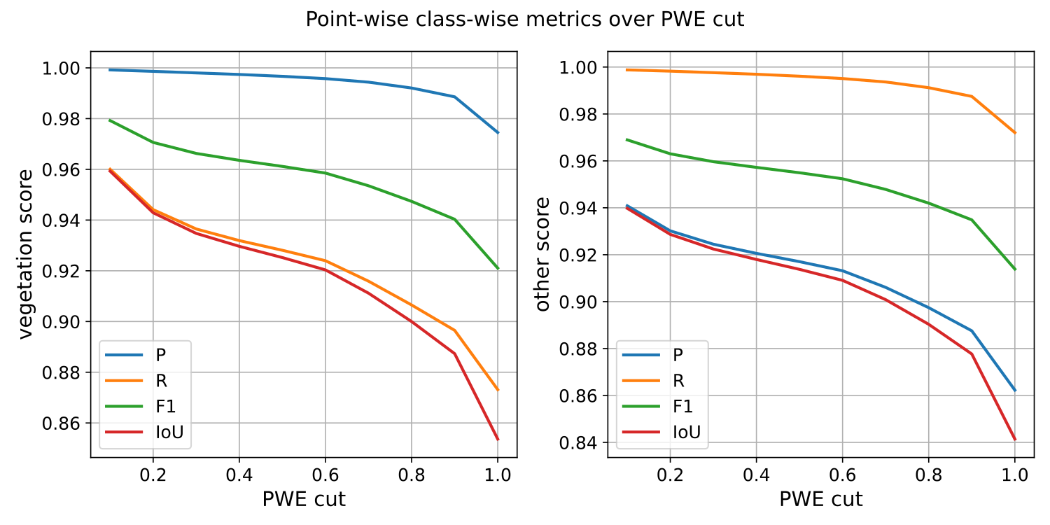
The class-wise evaluation as a function of the point-wise entropy exported by the advanced classification evaluator.

Classification uncertainty evaluator

The ClassificationUncertaintyEvaluator can be used to get insights on what points are more problematic for a given model when solving a particular point-wise classification task. The evaluation will be more detailed when there is more data available (e.g., reference labels) but it can also be computed solely from the predicted probabilities. A ClassificationUncertaintyEvaluator can be defined inside a pipeline using the JSON below:

{
    "eval": "ClassificationUncertaintyEvaluator",
    "class_names": ["Ground", "Vegetation", "Building", "Urban furniture", "Vehicle"],
    "include_probabilities": true,
    "include_weighted_entropy": true,
    "include_clusters": true,
    "weight_by_predictions": false,
    "num_clusters": 10,
    "clustering_max_iters": 128,
    "clustering_batch_size": 1000000,
    "clustering_entropy_weights": true,
    "clustering_reduce_function": "mean",
    "gaussian_kernel_points": 256,
    "report_path": "uncertainty/uncertainty.las",
    "plot_path": "uncertainty/"
}

The JSON above defines a ClassificationUncertaintyEvaluator that will export a point cloud and many plots to the uncertainty directory.

Arguments

– class_names

A list with the names for the classes. These names will be used to represent the classes in the plots and the reports.

– ignore_classes

Optional list of classes to be ignored when computing the uncertainty metrics. Any point whose label matches a class in this list will be excluded. The classes must be given as a list of strings that matches those from class_names, i.e., ignore_classes \(\subseteq\) class_names.

– probability_eps

A value representing the zero. It can be useful to avoid NaNs when computing the logarithms of the likelihoods, i.e., \(\log_2(0)\). If it is exactly zero, then logarithms of zero might arise. Otherwise, the zeroes will be replaced by this value or the minimum greater than zero likelihood, whatever is smaller.

– include_probabilities

Whether to include the probabilities in the output point cloud (True) or not (False).

– include_weighted_entropy

Whether to include the weighted entropy in the evaluation (True) or not (False). The weighted entropy considers either the distribution of reference or predicted labels to compensate for unbalanced class distributions.

– include_clusters

Whether to include the cluster-wise entropy in the evaluation (True) or not (False). Note that the cluster-wise entropy might take too long to compute depending on how it is configured.

– weight_by_predictions

Whether to compute the weighted entropy considering the predictions instead of the reference labels (True) or not (False, by default).

– num_clusters

How many clusters must be computed for the cluster-wise entropy.

– clustering_max_iters

How many iterations are allowed at most when computing the clustering algorithm (KMeans).

– clustering_batch_size

How many points per batch must be considered when computing the batch KMeans.

– clustering_entropy_weights

Whether to use point-wise entropy as the sample weights for the KMeans clustering (True) or not (False).

– clustering_reduce_function

What function must be used to reduce all the entropies in a given cluster to a single one that will be assigned to all points in the cluster. Supported reduce functions are:

• "mean" Select the mean entropy value.

• "median" Select the median of the entropy distribution.

• "Q1" Select the first quartile of the entropy distribution.

• "Q3" Select the third quartile of the entropy distribution.

• "min" Select the min entropy value.

• "max" Select the max entropy value.

– gaussian_kernel_points

How many points will be considered to evaluate each gaussian kernel density estimation.

– report_path

Path to write the point cloud with the computed uncertainty metrics.

– plot_path

Path to the directory where the many plots representing the computed uncertainty metrics will be written.

Output

The output is illustrated considering the March 2018 point clouds from the Hessigheim dataset to compute the classification’s uncertainty evaluation.

Below, an example of one of the figures that can be generated with the ClassificationUncertaintyEvaluator. It clearly illustrates that the point-wise classification of vehicles is problematic.

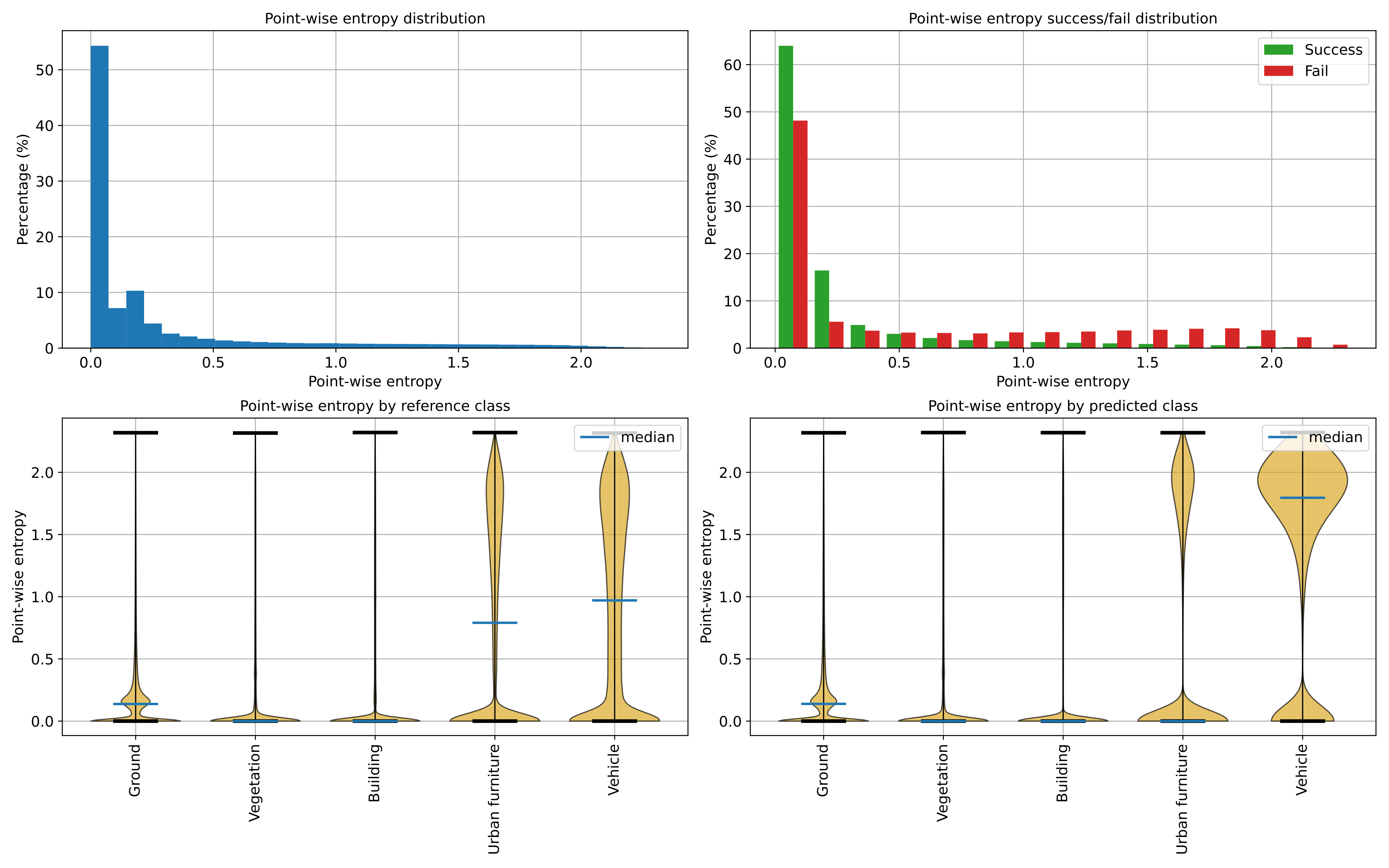
Visualization of the point-wise entropy outside the point cloud.

Below, an example of the point cloud representing the uncertainty metrics. In the general case, it can be seen that a high class ambiguity is associated with misclassified points. Thus, even in the absence of labeled point clouds, the uncertainty metrics can be used to understand the problems of a model when classifying previously unseen data.

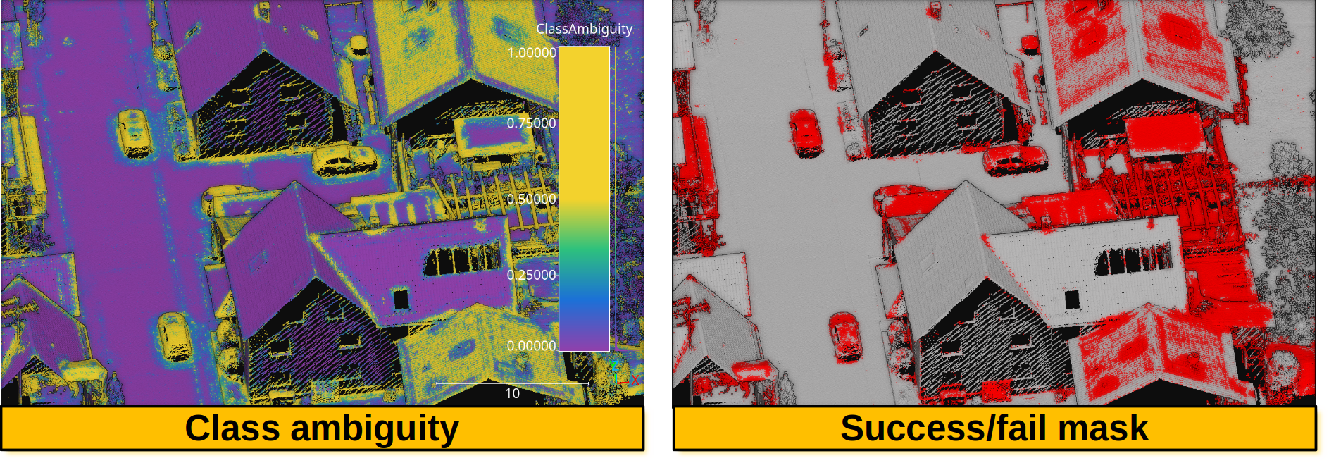
Visualization of a point cloud representing the class ambiguity and the success/fail point-wise mask on previously unseen data, respectively. Red means failed classification and gray means successfully classified.

Regression evaluator

The RegressionEvaluator assesses the relationship between numerical quantities assuming there is a reference one, therefore enabling error measurements. A RegressionEvaluator can be defined inside a pipeline using the JSON below:

{
    "eval": "RegressionEvaluator",
    "metrics": [
        "MSE", "RMSE", "MAE",
        "MaxSE", "RMaxSE", "MaxAE",
        "MinSE", "RMinSE", "MinAE",
        "MeSE", "RMeSE", "MeAE",
        "DevSE", "RDevSE", "DevAE",
        "RangeSE", "RRangeSE", "RangeAE",
        "Q1SE", "RQ1SE", "Q1AE",
        "Q3SE", "RQ3SE", "Q3AE",
        "SkSE", "SkAE",
        "KuSE", "KuAE",
        "Pearson", "Spearman"
    ],
    "cases": [
        ["sage_gauss_curv", "full_gauss_r0_4", "cc_Gauss_curv_r0_4"],
        ["sage_mean_curv", "full_mean_r0_4", "cc_Mean_curv_r0_4"],
        ["sage_shape_index", "shape_index_r0_4"],
        ["sage_umbildev", "umbilic_dev_r0_4"],
        ["sage_minabscurv", "minabscurv_r0_4"],
        ["sage_maxabscurv", "maxabscurv_r0_4"]
    ],
    "cases_renames":[
        ["GaussC", "ccGaussC"],
        ["MeanC", "ccMeanC"],
        ["Shpidx"],
        ["Umbdev"],
        ["minabsC"],
        ["maxabsC"]
    ],
    "outer_correlations": {
        "GaussC": {
            "abs_algdist_r0_4":{
                "metrics": ["SE", "AE"],
                "correlations": ["pearson", "spearman"],
                "frenames": ["GaussC_absad_SE_r", "GaussC_absad_SE_rho", "GaussC_absad_AE_r", "GaussC_absad_AE_rho"]
            },
            "linear_norm_r0_4":{
                "metrics": ["SE", "AE"],
                "correlations": ["pearson", "spearman"],
                "frenames": ["GaussC_lnorm_SE_r", "GaussC_lnorm_SE_rho", "GaussC_lnorm_AE_r", "GaussC_lnorm_AE_rho"]
            },
            "full_gradnorm_r0_4":{
                "metrics": ["SE", "AE"],
                "correlations": ["pearson", "spearman"],
                "frenames": ["GaussC_gnorm_SE_r", "GaussC_gnorm_SE_rho", "GaussC_gnorm_AE_r", "GaussC_gnorm_AE_rho"]
            }
        },
        "ccGaussC": {
            "abs_algdist_r0_4":{
                "metrics": ["SE", "AE"],
                "correlations": ["pearson", "spearman"],
                "frenames": ["ccGaussC_absad_SE_r", "ccGaussC_absad_SE_rho", "ccGaussC_absad_AE_r", "ccGaussC_absad_AE_rho"]
            },
            "linear_norm_r0_4":{
                "metrics": ["SE", "AE"],
                "correlations": ["pearson", "spearman"],
                "frenames": ["ccGaussC_lnorm_SE_r", "ccGaussC_lnorm_SE_rho", "ccGaussC_lnorm_AE_r", "ccGaussC_lnorm_AE_rho"]
            },
            "full_gradnorm_r0_4":{
                "metrics": ["SE", "AE"],
                "correlations": ["pearson", "spearman"],
                "frenames": ["ccGaussC_gnorm_SE_r", "ccGaussC_gnorm_SE_rho", "ccGaussC_gnorm_AE_r", "ccGaussC_gnorm_AE_rho"]
            }
        },
        "MeanC": {
            "abs_algdist_r0_4":{
                "metrics": ["SE", "AE"],
                "correlations": ["pearson", "spearman"],
                "frenames": ["MeanC_absad_SE_r", "MeanC_absad_SE_rho", "MeanC_absad_AE_r", "MeanC_absad_AE_rho"]
            },
            "linear_norm_r0_4":{
                "metrics": ["SE", "AE"],
                "correlations": ["pearson", "spearman"],
                "frenames": ["MeanC_lnorm_SE_r", "MeanC_lnorm_SE_rho", "MeanC_lnorm_AE_r", "MeanC_lnorm_AE_rho"]
            },
            "full_gradnorm_r0_4":{
                "metrics": ["SE", "AE"],
                "correlations": ["pearson", "spearman"],
                "frenames": ["MeanC_gnorm_SE_r", "MeanC_gnorm_SE_rho", "MeanC_gnorm_AE_r", "MeanC_gnorm_AE_rho"]
            }
        },
        "ccMeanC": {
            "abs_algdist_r0_4":{
                "metrics": ["SE", "AE"],
                "correlations": ["pearson", "spearman"],
                "frenames": ["ccMeanC_absad_SE_r", "ccMeanC_absad_SE_rho", "ccMeanC_absad_AE_r", "ccMeanC_absad_AE_rho"]
            },
            "linear_norm_r0_4":{
                "metrics": ["SE", "AE"],
                "correlations": ["pearson", "spearman"],
                "frenames": ["ccMeanC_lnorm_SE_r", "ccMeanC_lnorm_SE_rho", "ccMeanC_lnorm_AE_r", "ccMeanC_lnorm_AE_rho"]
            },
            "full_gradnorm_r0_4":{
                "metrics": ["SE", "AE"],
                "correlations": ["pearson", "spearman"],
                "frenames": ["ccMeanC_gnorm_SE_r", "ccMeanC_gnorm_SE_rho", "ccMeanC_gnorm_AE_r", "ccMeanC_gnorm_AE_rho"]
            }
        },
        "Shpidx": {
            "abs_algdist_r0_4":{
                "metrics": ["AE"],
                "correlations": ["pearson", "spearman"],
                "frenames": ["Shpidx_absad_AE_r", "Shpidx_absad_AE_rho"]
            },
            "full_gradnorm_r0_4":{
                "metrics": ["AE"],
                "correlations": ["pearson", "spearman"],
                "frenames": ["Shpidx_gnorm_AE_r", "Shpidx_gnorm_AE_rho"]
            }
        },
        "Umbdev": {
            "abs_algdist_r0_4":{
                "metrics": ["AE"],
                "correlations": ["pearson", "spearman"],
                "frenames": ["Umbdev_absad_AE_r", "Umbdev_absad_AE_rho"]
            },
            "full_gradnorm_r0_4":{
                "metrics": ["AE"],
                "correlations": ["pearson", "spearman"],
                "frenames": ["Umbdev_gnorm_AE_r", "Umbdev_gnorm_AE_rho"]
            }
        },
        "minabsC": {
            "abs_algdist_r0_4":{
                "metrics": ["AE"],
                "correlations": ["pearson", "spearman"],
                "frenames": ["minabsC_absad_AE_r", "minabsC_absad_AE_rho"]
            },
            "full_gradnorm_r0_4":{
                "metrics": ["AE"],
                "correlations": ["pearson", "spearman"],
                "frenames": ["minabsC_gnorm_AE_r", "minabsC_gnorm_AE_rho"]
            }
        },
        "maxabsC": {
            "abs_algdist_r0_4":{
                "metrics": ["AE"],
                "correlations": ["pearson", "spearman"],
                "frenames": ["maxabsC_absad_AE_r", "maxabsC_absad_AE_rho"]
            },
            "full_gradnorm_r0_4":{
                "metrics": ["AE"],
                "correlations": ["pearson", "spearman"],
                "frenames": ["maxabsC_gnorm_AE_r", "maxabsC_gnorm_AE_rho"]
            }
        }
    },
    "outlier_filter": null,
    "outlier_param": 0,
    "regression_report_path": "*/report/regression_eval.log",
    "outer_report_path": "*/report/outer_eval.log",
    "distribution_report_path": "*/report/regression_distrb.log",
    "regression_pcloud_path": "*/report/regression_eval.las",
    "regression_plot_path": "*/plot/regression_plot.png",
    "regression_hist2d_path": "*/plot/regression_hist2d.png",
    "residual_plot_path": "*/plot/residual_plot.png",
    "residual_hist2d_path": "*/plot/residual_hist2d.png",
    "scatter_plot_path": "*/plot/scatter_plot.png",
    "scatter_hist2d_path": "*/plot/scatter_hist2d.png",
    "qq_plot_path": "*/plot/qq_plot.png",
    "summary_plot_path": "*/plot/summary_plot.png",
    "nthreads": -1
}

The JSON above defines a RegressionEvaluator that will consider the analytical Gaussian and mean curvatures, shape index, umbilical deviation and absolute curvatures computed with Sagemath. These reference values will be used to compute the Mean Squared Error ("MSE"), Root Mean Squared Error ("RMSE"), Mean Absolute Error ("MAE"), the Median Absolute Error ("MeAE"), and many more metrics for the curvature values computed with the geometric eatures miner++ of the VL3D++ framework. Moreover, the correlations between the errors on the estimated curvatures and some arbitrary geometric properties will be computed too. Note that, in this case, there is no outlier filtering at all.

Arguments

– metrics

A list with the names of the metrics that can be computed. Metrics based on error (i.e., raw diferences) are ["ME", "MaxE", "MinE", "MeE", "DevE", "RangeE", "Q1E", "Q3E", "SkE", "KuE"], those based on the squared error are ["MSE", "MaxSE", "MinSE", "MeSE", "DevSE", "RangeSE", "Q1SE", "Q3SE", "SkSE", "KuSE"], those based on the root of some aggregation of the squared error ["RMSE", "RMaxSE", "RMinSE", "RMeSE", "RDevSE", "RRangeSE", "RQ1SE", "RQ3SE"], and those based on the absolute error are ["MAE", "MaxAE", "MinAE", "MeAE", "DevAE", "RangeAE", "Q1AE", "Q3AE", "SkAE", "KuAE"], . Note that the metric name format convention is "Mx" mean of x, "Maxx" max of x, "Minx" min of x, "Mex" median of x, "Devx" standard deviation of x, "Rangex" range of x, "Q1x" first quartile of x, "Q3x" third quartile of x, "Skx" skewness of x, "Kux" kurtosis of x. Besides, ["Pearson", "Spearman"] correlations can be computed, which automatically involves computing associated \(p\)-values too.

– cases

A list of lists. Each inner list uses the first element to specify the reference attribute and following elements specify the different predicted attributes whose error must be measured with respect to the references.

– cases_renames

A list of lists. Each inner list must have as many elements as each inner in cases minus one. Each element must be a string uniquely naming the metrics computed for the case.

– outer_correlations

A dictionary whose keys are the case names (as specified through cases_renames) and whose values are another dictionary. Each subdictionary has as keys the names of the features (that must be available in the point cloud at the current time in the pipeline) whose correlations must be computed. The values of the each subdictionary are another dictionary with three elements:

– metrics

A list specifying the error metrics that must be considered for the correlations. Supported ones are the raw error "E", the squared error "SE", and the absolute error "AE".

– correlations

A list specifying the correlations that must be computed. Supported ones are "pearson" (linear relationship) and "spearman" (monotonic relationship).

– frenames

For each error metric and each correlation (iterated with nested loops in the same order as mentioned) the name of the resulting measurement.

– outlier_filter

What outlier filtering strategy must be applied. If not given, then outliers are not filtered. Supported strategies are \(k\) times the standard deviation ("stdev"), \(k\) times the interquartile range minus the first quartiles and plus the third quartile ("iqr"), discard top \(k\) errors ("topk"), discard bottom \(k\) errors ("botk"), discard top and bot k errors (extremek), discard \(p\) percentage of greatest errors ("topp"), discard \(p\) percentage of least errors ("botp"), and discard \(p\) percentage of greateast and least errors ("extremp").

– outlier_param

The parameter governing the outlier filter (e.g., \(k\) for the "stdev" outlier filter.

– regression_report_path

Path to write the report with the regression metrics to a text file.

– outer_report_path

Path to write the report with the correlations to a text file.

– distribution_report_path

Path to write the report with the percentiles for each feature (including references, predictions, and arbitrary features involved in the correlations).

– regression_pcloud_path

Path to write the point cloud with the point-wise error measurements.

– regression_plot_path

Path to write the residual scatter plot with the predictions on the \(x\)-axis and the error on the \(y\)-axis.

– regression_hist2d_path

Path to write a 2D histogram representation of the residuals. It is similar to the plot generated for regression_plot_path but accounting for the density through the color.

– residual_plot_path

Path to write the residual scatter plot with the references on the \(x\)-axis and the error on the \(y\)-axi.

– residual_hist2d_path

Path to write a 2D histogram representation of the residuals. It is similar to the plot generated for residual_plot_path but accounting for the density through the color.

– scatter_plot_path

The scatter plot for the different features involved in the error metrics and correlations.

– scatter_hist2d_path

Path to write a 2D histogram representation of the correlation between pairs of features. It is similar to the plot generated by scatter_plot_path but accounting for the density through the color.

– qq_plot_path

Path to write the QQ plot for each pair (reference, prediction) involved in the computation of the error metrics.

– summary_plot_path

Path to write a plot summarizing the mean and standard deviation of each regression.

– nthreads

How many threads must be used in parallel computations. NOTE that currently, parallelism is not supported for RegressionEvaluator.

Output

The output is illustrated considering an hyperbolic paraboloid and a torus.

The table below represents the mean absolute error (MAE), median absolute error (MeAE), standard deviation of absolute error (DevAE), max absolute error (MaxAE), mean squared error (MSE), median squared error (MeSE), standard deviation of squared error (DevSE), max squared error (MaxSE), Pearson correlation coefficient, and Spearman correlation coefficient.

Feature	MAE	MeAE	DevAE	MaxAE	MSE	MeSE	DevSE	MaxSE	Pearson	Spearman
GaussC	0.01588	0.01349	0.01208	0.06843	0.00040	0.00018	0.00057	0.00468	0.99976	0.99939
MeanC	0.01172	0.01001	0.00928	0.07289	0.00022	0.00010	0.00040	0.00531	0.99166	0.99200
Shpidx	0.00918	0.00723	0.00890	0.06722	0.00016	0.00005	0.00037	0.00452	0.99386	0.99487
Umbdev	0.01741	0.01405	0.01575	0.25869	0.00055	0.00020	0.00198	0.06692	0.99955	0.99945
minabsC	0.01365	0.01089	0.01053	0.07488	0.00030	0.00012	0.00042	0.00561	0.99935	0.99957
maxabsC	0.01463	0.01063	0.01455	0.20185	0.00043	0.00011	0.00131	0.04074	0.99858	0.99897

The image belows represents the point-wise mean curvature and shape index for the hyperbolic paraboloid and the torus, respectively. Besides the corresponding absolute and squared errors.

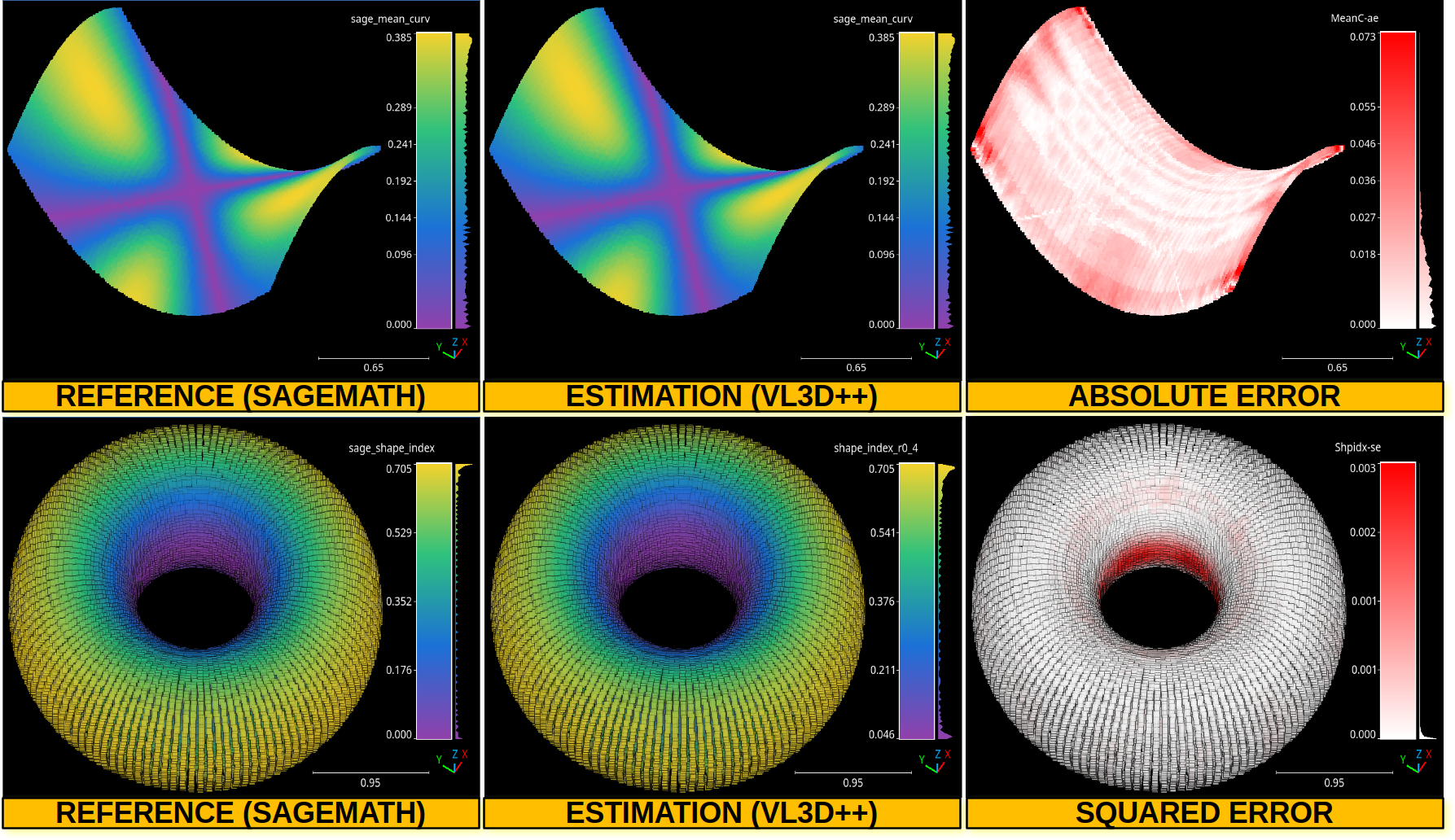
The top row shows the point-wise mean curvature and its absolute error on an hyperbolic paraboloid. The bottom row shows the point-wise shape index and its squared error on a torus.

Deep learning model evaluator

The DLModelEvaluator assumes there is a deep learning at the current pipeline’s state that can be used to process the point cloud at the current pipeline’s state. Instead of returning the output point-wise predictions, the values of the output layer and some internal feature representation will be returned to be visualized directly in the point cloud. Note that the internal feature representation might need an enormous amount of memory as it scales depending on how many features are generated by the architecture at the studied layer. A DLModelEvaluator can be defined inside a pipeline using the JSON below:

{
    "eval": "DLModelEvaluator",
    "pointwise_model_output_path": "pwise_out.las",
    "pointwise_model_activations_path": "pwise_activations.las"
}

The JSON above defines a DLModelEvaluator that will export the values of the output layer to the file pwise_out.las and a representation of the features in the hidden layers to the file pwise_activations.las.

Arguments

– pointwise_model_output_path

Where to export the point cloud with the point-wise outputs of the neural network.

– pointwise_model_activations_path

Where to export the point cloud with the internal features of the neural network.

Output

The output is illustrated considering the March 2018 point clouds from the Hessigheim dataset to compute the deep learning model evaluation. The figure below illustrates four different features extracted by the neural network. They are taken as the activated outputs of the last layer before the softmax .

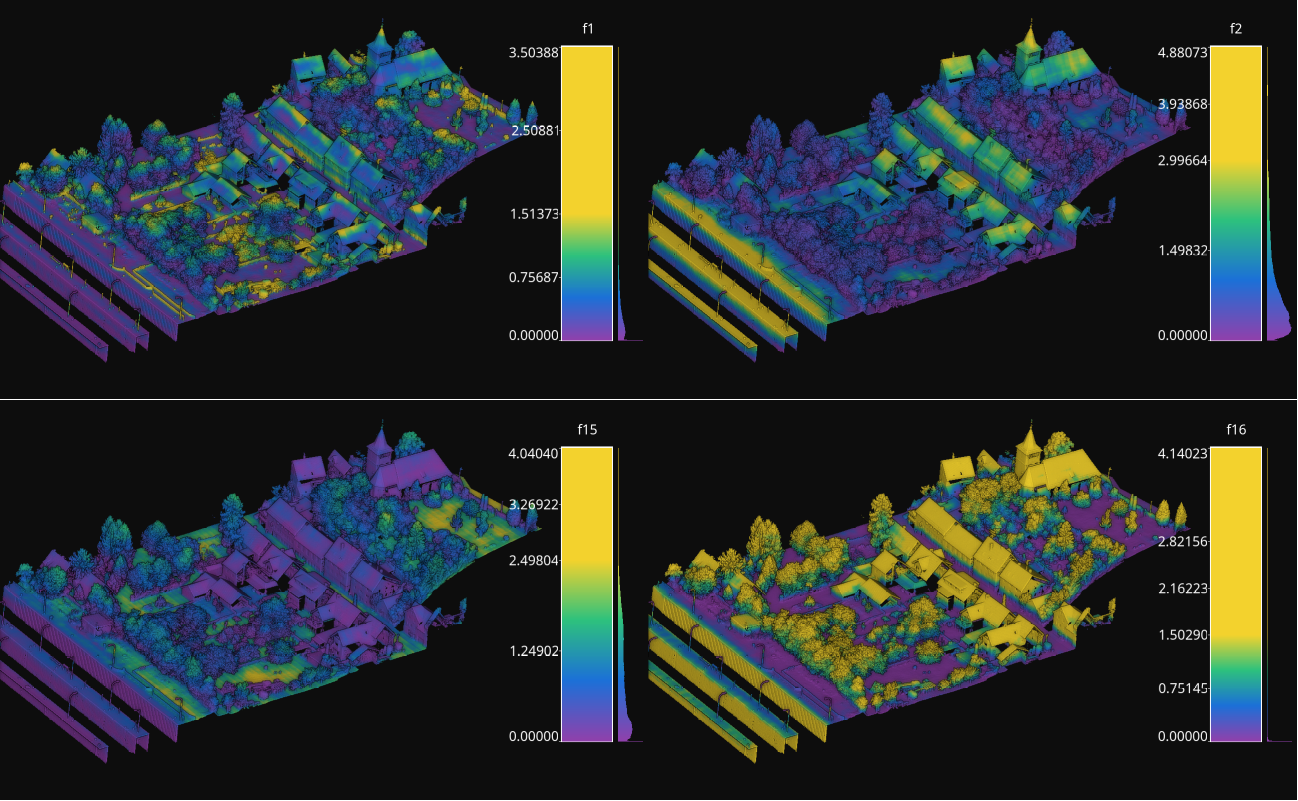
Visualization of some features used by a PointNet-based neural network for point-wise classification.

Raster grid evaluator

The RasterGridEvaluator can be used to evaluate the point cloud on a grid. This grid can later be exported to a GeoTIFF file that extends the grid with geographic information. Therefore, the GeoTIFF can be used to evaluate the features or classifications in the point cloud, e.g., loading the GeoTIFF in a GIS software to compare the rasterized point cloud with satellite image or maps in general. The GeoTIFFs are generated using the RasterIO library.

{
            "eval": "RasterGridEvaluator",
            "crs": "+proj=utm +zone=29 +ellps=GRS80 +towgs84=0,0,0,0,0,0,0 +units=m +no_defs +type=crs",
            "plot_path": "*geotiff/",
            "conditions": null,
            "xres": 1.0,
            "yres": 1.0,
            "grid_iter_step": 1024,
            "grids": [
                    {
                            "fnames": ["Vegetation"],
                            "reduce": "mean",
                            "empty_val": "nan",
                            "target_relational": "equals",
                            "oname": "vegetation_mean"
                    },
                    {
                            "fnames": ["Vegetation"],
                            "reduce": "max",
                            "empty_val": "nan",
                            "target_relational": "equals",
                            "oname": "vegetation_max"
                    },
                    {
                            "fnames": ["Prediction"],
                            "target_val": 2,
                            "target_relational": "equals",
                            "reduce": "binary_mask",
                            "count_threshold": 3,
                            "empty_val": "nan",
                            "oname": "vegetation_mask"
                    },
                    {
                            "fnames": ["Ground", "Vegetation", "Other"],
                            "reduce": "mean",
                            "empty_val": "nan",
                            "target_relational": "equals",
                            "oname": "GVO_mean"
                    },
                    {
                            "fnames": ["Ground", "Vegetation", "Other"],
                            "reduce": "max",
                            "empty_val": "nan",
                            "target_relational": "equals",
                            "oname": "GVO_max"
                    },
                    {
                            "fnames": ["PointWiseEntropy"],
                            "reduce": "mean",
                            "empty_val": "nan",
                            "target_relational": "equals",
                            "oname": "pwise_entropy_mean"
                    },
                    {
                            "fnames": ["PointWiseEntropy"],
                            "reduce": "max",
                            "empty_val": "nan",
                            "target_relational": "equals",
                            "oname": "pwise_entropy_max"
                    }
            ]
    }

The JSON above defines a RasterGridEvaluator that generates many GeoTIFFs using the EPSG:25829 coordinate reference system (specified using PROJ syntax). The GeoTIFFs are exported to the geotiff subdirectory, considering the output prefix of the pipeline. The cell size is \(1\,\mathrm{m}\) along each axis. Some GeoTIFFs use a single color channel to represent a continuous value. One particular GeoTIFF generates a binary mask for each cell with \(1\) when there are at least \(3\) points classified as vegetation and \(0\) otherwise. The GeoTIFFs that consider the likelihood for Ground, Vegetation, and Other classes will export each likelihood in a different color channel.

Arguments

– crs

The coordinate reference system specification. See the RasterIO documentation for more information about CRS specification.

– plot_path

The directory where the GeoTIFF files will be stored.

– conditions

A list with many conditions specified as dictionaries. These conditions will be applied to filter the entire point cloud before computing any raster or grid. See the advanced evaluator conditions documentation for further details.

– xres

The cell resolution along the x-axis.

– yres

The cell resolution along the y-axis.

– grid_iter_step

How many max rows per iteration. It can be tuned to improve the efficiency but also to prevent memory exhaustion.

– radius_expr

An optional specification to define the computation of the radius for the ball-like neighborhoods. The variable "l" represents the max cell size and it is the default radius expression. Note that any expression less than "sqrt(2)*l/2" (half of the cell’s hypotenuse) will potentially ignore some points inside the cell boundary. Also, values greater than the previous one will increase the “smooth” effect through more overlapped neighborhoods.

– grids

A list with potentially many grid specifications. A grid can be specified with a dictionary-like style:

{
    "fnames": ["feat1", "feat2"],
    "reduce": "mean",
    "empty_val": "nan",
    "target_relational": "equals",
    "target_val": 2,
    "count_threshold": 3,
    "oname": "my_geotiff"
}

The fnames list must specify the name of the involved features. It can be null but only when the reduce strategy is "binary_mask" (binary occupation mask, i.e., whether a cell contains at least one point or not), "recount" (number of points per cell) or "relative_recount" (normalized number of points per cell).

The optional conditions list must specify the conditional filters that must be applied to the data for a particular grid. Its specification is the same as for the advanced evaluator conditions.

The reduce string must refer to a strategy to reduce many values per cell to a single one, e.g., "mean", "median", "min", "max", "binary_mask", "recount", and "relative_recount".

The empty_val value will be assigned to represent the cells with no points. They can be numbers or the string "nan" (not a number).

The target_relational governs how the values will be compared against the target. Supported relationals are "equals" (\(=\)), "not_equals" (\(\neq\)), "less_than" (\(<\)), "less_than_or_equal_to" (\(\leq\)), "greater_than" (\(>\)), "greater_than_or_equal_to" (\(\geq\)), "in" (\(\in\)), and "not_in" (\(\notin\)). Note that it must be given even if not used.

The target_val the value that must be searched when using a binary mask strategy.

The count_threshold governs how many times the target value must be found to consider a \(1\) for the binary mask.

The dem overloads the previous specifications and instead computes a Digital Elevation Model (DEM) assuming the \((x, y)\) plane with elevation values corresponding to \(z\). Note that since all the other arguments are ignored, only the global conditions of the RasterGridEvaluator are applied. Post-processing interpolations are still possible but generally not especially useful as the DEM already involves a 2D grid interpolation. The DEM is computed through the DEMGenerator class. It supports selecting its internal interpolation strategy (either "linear", "nearest", or "cubic"), by default it is

"dem": {
    "interpolation": "linear"
}

The interpolator can post-process the generated raster to interpolate some cells considering the values in the others through radial basis functions. It is based on the GridInterpolator2D class. Below an example of a potential interpolator specificaiton for a particular grid:

"interpolator": {
    "iterations": 2,
    "domain": {
        "strategy": "polygonal_contour_target",
        "channel": 0,
        "erosions": 2,
        "dilations": 3,
        "polygonal_approximation": 0,
        "target_val": "nan",
        "target_relational": "equals"
    },
    "interpolation": {
        "smoothing": 0.0,
        "kernel": "linear",
        "neighbors": 64,
        "epsilon": null,
        "degree": null,
        "clip_interval": [0, null]
    }
}

The arguments of the interpolator are:

– iterations

How many times apply the entire interpolation strategy to the grid.

– domain

The specification of the first stage where the cells that must be interpolated are determined. Its arguments are:

– strategy

The strategy to determine the cells to be interpolated. It can be: "all" to interpolate all the cells in the grid, "target" to interpolate only the cells in the grid that satisfy the given relational, "polygonal_contour" to interpolate all the cells in the grid inside the region closed by the contour of the cells that do not satisfy the given relational, or "polygonal_contour_target" to interpolate only the cells that satisfy the given relational and are inside the region closed by the contour of the cells that do not satisfy the given relational.

– channel

The channel (default 0) that must be selected when the grid contains many values per cell to check the relational.

– erosions

How many morphological erosions perform before computing the contour (see scikit-image documentation about erosion).

– dilations

How many morphological dilations perform after the erosions but before computing the contour (see scikit-image documentation about dilation).

– polygonal_approximation

The tolerance for the polygonal approximation using the Douglas-Peucker algorithm. Note that if zero is given there is no polygonal approximation at all. (see scikit-image documentation about approximate polygons).

– target_val

The target value for the relational check. Typically, it will be a number. However, it can be a list given the two endpoints of the interval for "inside_open" and "inside_close" relationals or a list representing the items of a set for "in" and "not_in" relationals.

– target_relational

The relational itself. It can be either "equals" (\(=\)), "not_equals" (\(\neq\)), "less_than" (\(<\)), "less_than_or_equal_to" (\(\leq\)), "greater_than" (\(>\)), "greater_than_or_equal_to" (\(\geq\)), "inside_open" (\(\in (a, b)\)), "inside_close" (\(\in [a, b]\)), "in" (\(\in\)), or "not_in" (\(\notin\)).

– interpolation

The specification of the second stage where the cells that must be interpolated are effectively interpolated.

– kernel

See the kernel parameter in the SciPy documentation.

– smoothing

See the smoothing parameter in the SciPy documentation.

– neighbors

See the neighbors parameter in the SciPy documentation.

– epsilon

See the epsilon parameter in the SciPy documentation.

– degree

See the degree parameter in the SciPy documentation.

– clip_interval

If given, it must be a list of exactly two elements. The first element is the min value such that any value in the grid that is below it will be set to the min value. The second element is the max value such that any value in the grid that is above it will be set to the max value. One of the elements in this list can be null. In that chase, no clipping to that endpoint will be applied.

The hillshading specification, as a post-processing step to improve the visibility of certain landforms in the output raster. Below an example of the hillshading post-processing with default values:

"hillshading": {
    "azimuth": 30,
    "altitude": 30
}

The arguments for the hillshading specification are:

– azimuth

The angle of the light source with respect to the surface. It must be inside \([0, 360)\) degrees.

—altitude The angle where the light source is located. It must be inside \([0, 90]\) degrees.

The oname name for the output GeoTIFF file corresponding to the grid specification.

– reverse_rows

Boolean flag to control whether to reverse the rows of the grid (True) or not (False). The default is the reversed order, i.e., True.

– nthreads

The number of threads for the parallel computation of the grids. By default, just one thread is used. The value -1 implies using as many threads as available cores.

Output

The output is illustrated considering some MLS points clouds acquired in the region of Pontevedra, Galicia, northwest Spain. The points sum up to \(6.15 \times 10^{8}\) from a dataset of \(3.51 \times 10^{9}\) points.

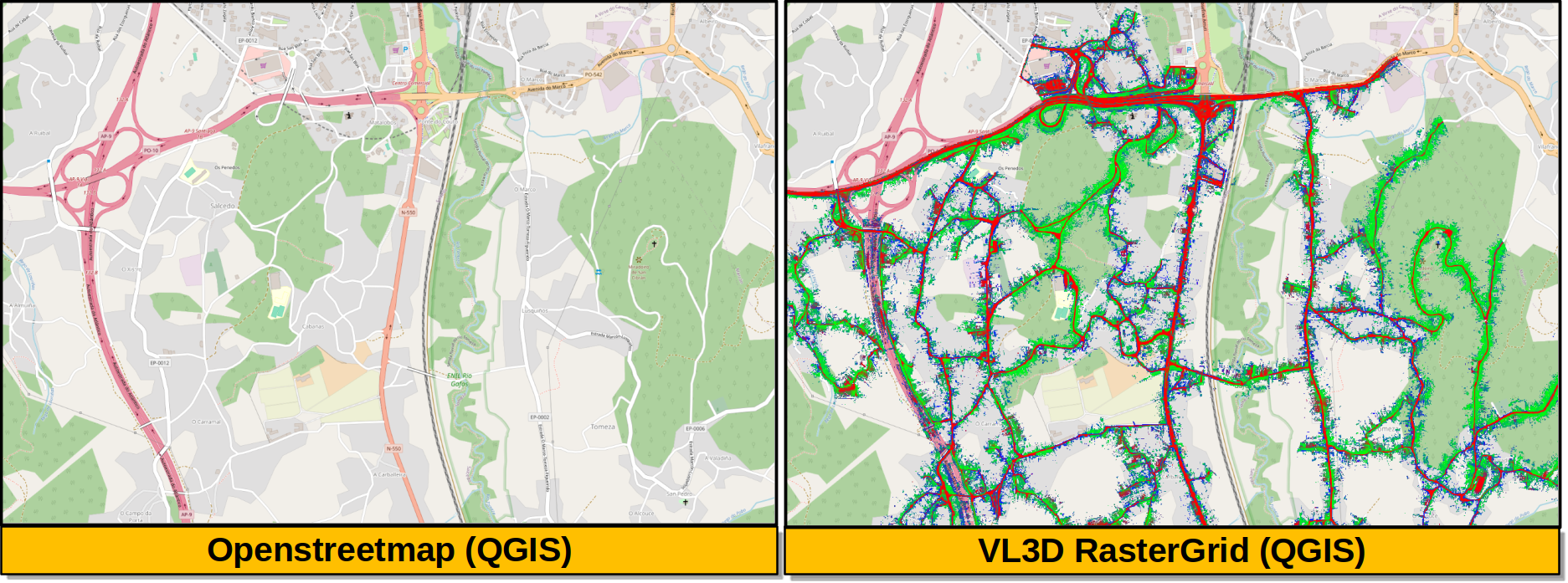
Visualization of the output GeoTIFFs on QGIS as an overlay to the Openstreetmap of the region of Pontevedra in Galicia, northwest Spain. The red color represents the mean ground likelihood in the neighborhood, green the vegetation likelihood, and blue any other class (e.g., buildings and powerlines).