Introduction
The VirtuaLearn3D++ (VL3D++) framework is a software for point-wise classification and regression on 3D point clouds. It handles the training and prediction operations of the many implemented models. On top of that, it provides useful tools for transforming the point clouds and for automatic feature extraction. Moreover, it also supports evaluations on the data, the models, and the predictions. These evaluations yield further insights and analysis through automatically generated plots, CSV files, text reports, and point clouds.
This framework is a fork of the VirtuaLearn3D (VL3D) framework originally developed in the context of the VirtuaLearn3D project of the 3DGeo research group funded by the German Research Foundation (DFG).
The VL3D++ framework is designed so the user can easily decide about the model configuration and define custom pipelines. To achieve this, the user only needs to manipulate JSON files like the one shown below:
{
  "in_pcloud": [
    "https://3dweb.geog.uni-heidelberg.de/trees_leafwood/PinSyl_KA10_03_2019-07-30_q2_TLS-on_c_t.laz"
  ],
  "out_pcloud": [
    "out/Geometric_PCA_RF_on_PinSyl_KA10_03/*"
  ],
  "sequential_pipeline": [
    {
      "miner": "GeometricFeatures",
      "radius": 0.05,
      "fnames": ["linearity", "planarity", "surface_variation", "eigenentropy", "omnivariance", "verticality", "anisotropy"]
    },
    {
      "miner": "GeometricFeatures",
      "radius": 0.1,
      "fnames": ["linearity", "planarity", "surface_variation", "eigenentropy", "omnivariance", "verticality", "anisotropy"]
    },
    {
      "miner": "GeometricFeatures",
      "radius": 0.2,
      "fnames": ["linearity", "planarity", "surface_variation", "eigenentropy", "omnivariance", "verticality", "anisotropy"]
    },
    {
      "writer": "Writer",
      "out_pcloud": "*pcloud/geomfeats.las"
    },
    {
      "imputer": "UnivariateImputer",
      "fnames": ["AUTO"],
      "target_val": "NaN",
      "strategy": "mean",
      "constant_val": 0
    },
    {
      "feature_transformer": "Standardizer",
      "fnames": ["AUTO"],
      "center": true,
      "scale": true
    },
    {
      "feature_transformer": "PCATransformer",
      "out_dim": 0.99,
      "whiten": false,
      "random_seed": null,
      "fnames": ["AUTO"],
      "report_path": "*report/pca_projection.log",
      "plot_path": "*plot/pca_projection.svg"
    },
    {
      "writer": "Writer",
      "out_pcloud": "*pcloud/geomfeats_transf.las"
    },
    {
      "train": "RandomForestClassifier",
      "fnames": ["AUTO"],
      "training_type": "stratified_kfold",
      "random_seed": null,
      "shuffle_points": true,
      "num_folds": 5,
      "model_args": {
        "n_estimators": 4,
        "criterion": "entropy",
        "max_depth": 20,
        "min_samples_split": 5,
        "min_samples_leaf": 1,
        "min_weight_fraction_leaf": 0.0,
        "max_features": "sqrt",
        "max_leaf_nodes": null,
        "min_impurity_decrease": 0.0,
        "bootstrap": true,
        "oob_score": false,
        "n_jobs": 4,
        "warm_start": false,
        "class_weight": null,
        "ccp_alpha": 0.0,
        "max_samples": 0.8
      },
      "autoval_metrics": ["OA", "P", "R", "F1", "IoU", "wP", "wR", "wF1", "wIoU", "MCC", "Kappa"],
      "stratkfold_report_path": "*report/RF_stratkfold_report.log",
      "stratkfold_plot_path": "*plot/RF_stratkfold_plot.svg",
      "hyperparameter_tuning": {
        "tuner": "GridSearch",
        "hyperparameters": ["n_estimators", "max_depth", "max_samples"],
        "nthreads": -1,
        "num_folds": 5,
        "pre_dispatch": 8,
        "grid": {
            "n_estimators": [2, 4, 8, 16],
            "max_depth": [15, 20, 27],
            "max_samples": [0.6, 0.8, 0.9]
        },
        "report_path": "*report/RF_hyper_grid_search.log"
      },
      "importance_report_path": "*report/LeafWood_Training_RF_importance.log",
      "importance_report_permutation": true,
      "decision_plot_path": "*plot/LeafWood_Training_RF_decission.svg",
      "decision_plot_trees": 3,
      "decision_plot_max_depth": 5
    },
    {
      "writer": "PredictivePipelineWriter",
      "out_pipeline": "*pipe/LeafWood_Training_RF.pipe",
      "include_writer": false,
      "include_imputer": true,
      "include_feature_transformer": true,
      "include_miner": true
    }
  ]
}
The JSON above defines a pipeline to train random forest models. It will download a labeled point cloud representing the PinSyl_KA10 tree to train a machine learning model. First, three sets of geometric features are computed with different radii. The generated features are then written to an output point cloud geomfeats.las to visualize them (see the geometric features miner documentation). The mean value of the feature will replace any feature with an invalid numerical value through the univariate imputer (see the univariate imputer documentation). Afterward, the features are standardized to have mean zero and standard deviation one (see the standardizer documentation). Then, the dimensionality of the feature space is transformed through PCA (see the PCA transformer documentation), and the resulting transformed features are exported to geomfeats_transf.las for visualization.
At this point, the features are used to train a random forest classifier (see the random forest classifier documentation). Using a stratified K-folding training strategy with \(K=5\) (see the stratified K-folding documentation). The trained model is evaluated through metrics like Overall Accuracy (OA) or Matthews Correlation Coefficient (MCC). Some model hyperparameters, like the number of estimators or the max depth of each decision tree, are explored using a grid search algorithm (see the grid search documentation). The best combination of hyperparameters is automatically selected to train the final model. Finally, the data mining, imputation, and feature transformation components are assembled with the random forest classifier, and serialized to a file LeafWood_Training_RF.pipe that can be later loaded to be used as a leaf-wood segmentation model.
Once a predictive pipeline has been exported (see the predictive pipeline documentation) it can be used as shown in the JSON below:
{
  "in_pcloud": [
    "https://3dweb.geog.uni-heidelberg.de/trees_leafwood/PinSyl_KA09_T048_2019-08-20_q1_TLS-on_c_t.laz"
  ],
  "out_pcloud": [
    "out/Geometric_PCA_RF_on_PinSyl_KA10_03/prediction/*"
  ],
  "sequential_pipeline": [
    {
      "predict": "PredictivePipeline",
      "model_path": "out/Geometric_PCA_RF_on_PinSyl_KA10_03/pipe/LeafWood_Training_RF.pipe"
    },
    {
      "writer": "ClassifiedPcloudWriter",
      "out_pcloud": "*predicted.las"
    },
    {
      "eval": "ClassificationEvaluator",
      "class_names": ["Wood", "Leaf"],
      "metrics": ["OA", "P", "R", "F1", "IoU", "wP", "wR", "wF1", "wIoU", "MCC", "Kappa"],
      "class_metrics": ["P", "R", "F1", "IoU"],
      "report_path": "*report/global_eval.log",
      "class_report_path": "*report/class_eval.log",
      "confusion_matrix_report_path" : "*report/confusion_matrix.log",
      "confusion_matrix_plot_path" : "*plot/confusion_matrix.svg",
      "class_distribution_report_path": "*report/class_distribution.log",
      "class_distribution_plot_path": "*plot/class_distribution.svg"
    },
    {
        "eval": "ClassificationUncertaintyEvaluator",
        "class_names": ["Wood", "Leaf"],
        "include_probabilities": true,
        "include_weighted_entropy": true,
        "include_clusters": true,
        "weight_by_predictions": false,
        "num_clusters": 10,
        "clustering_max_iters": 128,
        "clustering_batch_size": 1000000,
        "clustering_entropy_weights": true,
        "clustering_reduce_function": "mean",
        "gaussian_kernel_points": 256,
        "report_path": "*uncertainty/uncertainty.las",
        "plot_path": "*uncertainty/"
    }
  ]
}
The JSON above defines a pipeline to compute a leaf-wood segmentation based on a random forest model. It will download the PinSyl KA10 tree to compute the predictive pipeline. The predictions will be exported to the predicted.las point cloud. Furthermore, the point-wise classification can be evaluated because there are available labels on that tree (see the classification evaluator documentation). Afterward, the uncertainty of the classification is also evaluated (see the classification uncertainty evaluator documentation).
The figure below represents the previous process. It shows the training tree colored by the PCA-transformed feature which explains the highest variance ratio. It also shows the previously unseen tree as segmented by the model, with points colored gray if correctly classified or red if misclassified.
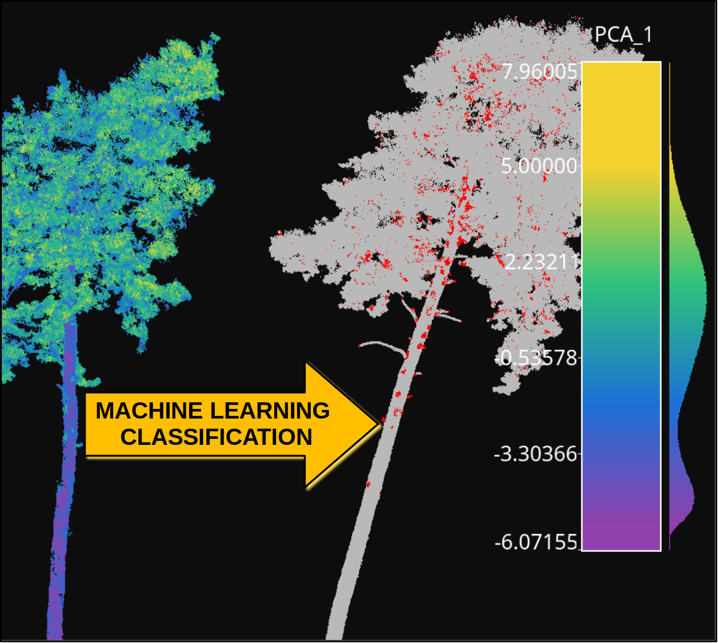
Visualization of a point-wise leaf-wood segmentation. The tree on the left side represents the training data, while the tree on the right side represents the leaf-wood segmentation computed on a previously unseen tree. The gray points are successful classifications, the red ones are misclassifications.
The table below represents the precision (P), recall (R), F1-score (F1), and the intersection over union or Jaccard index (IoU) of the leaf-wood segmentation represented in the figure above. The overall accuracy (OA) of the classification is around \(93\%\).
CLASS |
P |
R |
F1 |
IoU |
|---|---|---|---|---|
Wood |
93.952 |
84.073 |
88.738 |
79.756 |
Leaf |
92.986 |
97.501 |
95.190 |
90.822 |
You can automatically reproduce the explained model with the JSON specifications provided as a demo together with the source code in our GitHub repository. The first step is to get into the software directory. Then, for training you can run:
python vl3d.py --pipeline spec/demo/mine_transform_and_train_pipeline_pca_from_url.json
Finally, you can compute the point-wise segmentation on a previously unseen tree using:
python vl3d.py --pipeline spec/demo/predict_and_eval_pipeline_from_url.json