Pipelines
The VirtuaLearn3D (VL3D) framework supports the definition of pipelines combining different components into an ordered sequence of steps. Thus, it is possible to define a pipeline that mines features, selects the most convenient ones, and trains a machine learning model for point-wise classification tasks. Then, this pipeline can be exported as a predictive pipeline that can be applied to different point clouds.
Advanced input
Besides from the typical input specification for pipelines that consists of a list of paths to point clouds such that the pipeline will be run independently once for each point cloud, there are alternative input specifications that enable more complex input strategies.
Input point cloud concatenation
The input point cloud concatenation strategy supports merging many point
clouds into a single one, which can be useful -for example- to apply active
learning to datasets with many point clouds. In this case, the output must
be of a single element. Alternatively, the in_pcloud_concat can be a list
of lists. In this case, each inner list defines the point cloud involved
into a concatenation. There must be one output path for each inner list.
The list of dictionaries defining a concatenated point cloud considers the following arguments each:
- –
in_pcloud The path to the input point cloud.
- –
fnames The list with the names of the features that must be loaded. Note that it will only be considered for the first input point cloud, i.e.,
fnamesspecifications after the first point cloud will be ignored. If it is not given, then all the features available in the first point cloud will be considered.- –
offset A list with as many components as the dimensionality of the point cloud’s structure space (i.e., number of point-wise coordinates). When given, it will replace the offsets of the LAS header used to codify the point cloud in a binary format.
- –
mindist_decimator Optional specification to transform the input point cloud of \(m\) points to a transformed version of \(R \leq m\) points through the
MinDistDecimatorDecorator. The specification is similar to the minimum distance decimator decorated miner. Note that if bothmindist_decimatorandfps_transformerare given in the same specification, the minimum distance decimation is applied first, i.e., the FPS transformer will work on the decimated point cloud.- –
min_distance See the min_distance documentation of MinDistDecoratedMiner.
- –
num_encoding_neighbors See the num_encoding_neighbors documentation of MinDistDecoratedMiner.
- –
num_decoding_neighbors See the num_decoding_neighbors documentation of MinDistDecoratedMiner.
- –
release_encoding_neighborhoods See the release_encoding_neighborhoods documentation of MinDistDecoratedMiner.
- –
threads
- –
- –
fps_transformer Optional specification to transform the input point cloud of \(m\) points to a transformed version of \(R < m\) points through the
FPSDecoratorTransformer. The specification is similar to the FPS decorated model (FPSDecoratedModel) and the FPS decorated miner (FPSDecoratedMiner).- –
num_points The target number of points \(R\) for the transformed point cloud. It can be an integer or an expression that will be evaluated with \(m\) representing the number of points of the original point cloud, e.g.,
"m/2"will downscale the point cloud to half the number of points.- –
fast Whether to use exact furthest point sampling (
false) or a faster stochastic approximation (true).- –
num_encoding_neighbors How many closest neighbors in the original point cloud are considered for each point in the transformed point cloud to reduce from the original space to the transformed one.
- –
num_decoding_neighbors How many closest neighbors in the transformed point cloud are considered for each point in the original point cloud to propagate back from the transformed space to the original one.
- –
release_encoding_neighborhoods Whether the encoding neighborhoods can be released after computing the transformation (
true) or not (false). Releasing these neighborhoods means theFPSDecoratorTransformer.reduce()method must not be called, otherwise errors will arise. Setting this flag to true can help saving memory when needed.- –
threads The number of parallel threads to consider for the parallel computations. Note that
-1means using as many threads as available cores.
- –
- –
target_class_distribution A list specifying how many samples must be taken for each class. In case there are not enough points for a given class, the maximum possible number of points for that class will be considered.
- –
translation A list defining a translation vector of the same dimensionality as the structure space \(\pmb{u} \in \mathbb{R}^{n_x}\), i.e., with the same number of components/coordinates. This vector will be added to the coordinates of each point \(\pmb{x}_{i*} \in \mathbb{R}^{n_x}\) in the point cloud such that \(\pmb{x'}_{i*} = \pmb{x}_{i*} + \pmb{u}\).
- –
center A list defining the center point for the input point cloud. The coordinates of the points will be updated so the center of the point cloud, understood as the mid-range, matches the given center point. Note that if
translationis given then the center is not applied, i.e.,translationhas priority overcenter.
- –
conditions A list of dictionary-like conditions to filter the points before concatenating the point cloud. It is governed by four parameters:
value_nameThe name of the field to be considered (e.g., a feature name or the classification label).
condition_typeThe type of condition, i.e., the relational to be used. It can be
"not_equals"(\(\neq\)),"equals"(\(=\)),"less_than"(\(<\)),"less_than_or_equal_to"(\(\leq\)),"greater_than"(\(>\)),"greater_than_or_equal_to"(\(\geq\)),"in"\(\in\), and"not_in"\(\notin\).value_targetThe value target can be seen as the rhs of the relational when the value from the point cloud is represented as the lhs. For example, if \(x\) is the value from the point cloud, a relational could be \(x \notin S\) where \(S\) can be defined through the value target as
[0, 1, 3]. In this case, only the points with \(x \notin \{0, 1, 3\}\) will be considered.actionWhat must be done with the considered points. It can be either
"preserve"so the points that match the condition are preserved or"discard"to remove them.
The JSON below shows an example of how to use the input point cloud concatenation strategy. It was used to process a massive MLS dataset with active learning. The training dataset was derived as the concatenation between the point clouds labeled by the oracle. A visualization of the results is available in the raster grid evaluator’s documentation.
"in_pcloud_concat": [
    {
        "in_pcloud": "/hei/lidar_data/pontevedra/vl3d/training/T4/CANICOUVA.laz",
        "conditions": [
            {
                "value_name": "classification",
                "condition_type": "in",
                "value_target": [0, 1, 2],
                "action": "preserve"
            }
        ]
    },
    {
        "in_pcloud": "/hei/lidar_data/pontevedra/vl3d/training/T4/TOMEZA.laz",
        "conditions": [
            {
                "value_name": "classification",
                "condition_type": "in",
                "value_target": [0, 1, 2],
                "action": "preserve"
            }
        ]
    }
]
Sequential pipeline
A sequential pipeline is a connected sequence of components such that the component at \(t+1\) is executed on the state of the pipeline at \(t\) and potentially transforms it (depending on the component type).
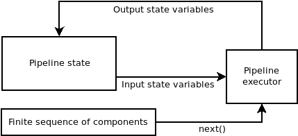
Diagram representing the logic of the sequential pipeline. The components are taken from the finite sequence until it has finished.
A sequential pipeline can be defined using JSON. First, let us start by how to specify the input and the output.
{
    "in_pcloud": ["/my/input/pcloud1.laz", "/my/input/pcloud2.laz"],
    "out_pcloud": ["/my/output/pcloud1/*", "/my/output/pcloud2/*"],
    "sequential_pipeline": []
}
In the JSON above, the in_pcloud key defines a list of input paths. In
general, these are expected to be point clouds in LAS or LAZ format. The
pipeline will be run independently one time for each point cloud in the input
list. Furthermore, the out_pcloud key defines a list of output paths. The
final asterisk ‘*’ at the end of these paths specifies that they will be
considered output prefixes. In other words, components that write some type
of output will append the output prefix to their paths (when they start by
another asterisk ‘*’). The interpretation of the JSON is that the output
generated by the pipeline when running on pcloud1.laz will be written to
/my/output/pcloud1/, while the output for pcloud2.laz will be written to
/my/output/pcloud2/.
Now, it is time to look at the sequential_pipeline specification. It must
be a list of components such that they will be executed in the same order
they are given. For example, it can be a sequence of two feature mining
components, followed by a writer to export the point cloud with features, an
imputer to handle numeric problems in the computed features, and
a Random Forest classifier, as shown in the JSON below:
{
  "in_pcloud": [
    "test_data/QuePet_BR01_01_2019-07-03_q2_TLS-on_c.laz",
    "test_data/test_tree.laz"
  ],
  "out_pcloud": [
    "out/training/sphinx/QuePet_BR01_kbest_RF/*",
    "out/training/sphinx/test_tree_kbest_RF/*"
  ],
  "sequential_pipeline": [
    {
      "miner": "GeometricFeatures",
      "radius": 0.05,
      "fnames": ["linearity", "planarity", "surface_variation", "eigenentropy", "omnivariance", "verticality", "anisotropy"],
      "frenames": ["linearity_r0_05", "planarity_r0_05", "surface_variation_r0_05", "eigenentropy_r0_05", "omnivariance_r0_05", "verticality_r0_05", "anisotropy_r0_05"]
    },
    {
      "miner": "GeometricFeatures",
      "radius": 0.1,
      "fnames": ["linearity", "planarity", "surface_variation", "eigenentropy", "omnivariance", "verticality", "anisotropy"],
      "frenames": ["linearity_r0_1", "planarity_r0_1", "surface_variation_r0_1", "eigenentropy_r0_1", "omnivariance_r0_1", "verticality_r0_1", "anisotropy_r0_1"]
    },
    {
      "writer": "Writer",
      "out_pcloud": "*pcloud/geomfeats.las"
    },
    {
      "imputer": "RemovalImputer",
      "target_val": "NaN",
      "fnames": ["AUTO"]
    },
    {
      "train": "RandomForestClassifier",
      "fnames": ["AUTO"],
      "training_type": "base",
      "random_seed": null,
      "model_args": {
        "n_estimators": 4,
        "criterion": "entropy",
        "max_depth": 20,
        "min_samples_split": 5,
        "min_samples_leaf": 1,
        "min_weight_fraction_leaf": 0.0,
        "max_features": "sqrt",
        "max_leaf_nodes": null,
        "min_impurity_decrease": 0.0,
        "bootstrap": true,
        "oob_score": false,
        "n_jobs": 4,
        "warm_start": false,
        "class_weight": null,
        "ccp_alpha": 0.0,
        "max_samples": 0.8
      }
    },
    {
      "writer": "PredictivePipelineWriter",
      "out_pipeline": "*pipe/LeafWood_Training_RF.pipe",
      "include_writer": false,
      "include_imputer": true,
      "include_feature_transformer": false,
      "include_miner": true,
      "include_class_transformer": false,
      "include_clustering": false,
      "ignore_predictions": false
    }
  ]
}
Finally, we can run the pipeline with a simple command (assuming our JSON file is named my_pipeline.json):
python3 vl3d.py --pipepline my_pipeline.json
As a result, we will obtain a predictive pipeline that can be used to compute point-wise leaf-wood segmentation on input point clouds. We will also obtain a point cloud that we can use to visualize the generated features. For example, the image below offers a visualization of the anisotropy for spherical negibhorhoods of \(10\,\mathrm{cm}\) radius.
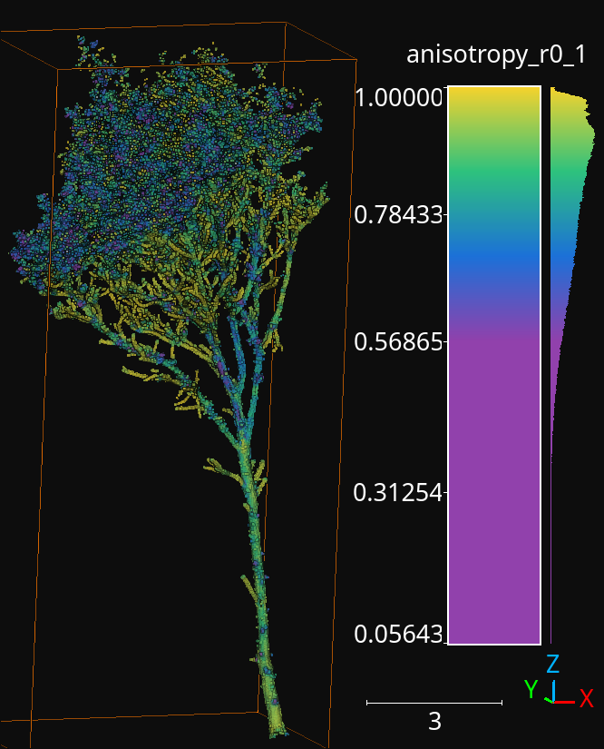
The anisotropy geometric feature computed during the execution of the pipeline for a radius of \(10\,\mathrm{cm}\).
Working example
The JSON below provides an example of a sequential pipeline to train a random forest for leaf-wood segmentation with more components. Pipelines like this one are more likely to arise during real data processing.
{
  "in_pcloud": [
    "test_data/QuePet_BR01_01_2019-07-03_q2_TLS-on_c.laz",
    "test_data/test_tree.laz"
  ],
  "out_pcloud": [
    "out/training/QuePet_BR01_kbest_RF/*",
    "out/training/test_tree_kbest_RF/*"
  ],
  "sequential_pipeline": [
    {
      "miner": "GeometricFeatures",
      "radius": 0.05,
      "fnames": ["linearity", "planarity", "surface_variation", "eigenentropy", "omnivariance", "verticality", "anisotropy"],
      "frenames": ["linearity_r0_05", "planarity_r0_05", "surface_variation_r0_05", "eigenentropy_r0_05", "omnivariance_r0_05", "verticality_r0_05", "anisotropy_r0_05"]
    },
    {
      "miner": "GeometricFeatures",
      "radius": 0.1,
      "fnames": ["linearity", "planarity", "surface_variation", "eigenentropy", "omnivariance", "verticality", "anisotropy"],
      "frenames": ["linearity_r0_1", "planarity_r0_1", "surface_variation_r0_1", "eigenentropy_r0_1", "omnivariance_r0_1", "verticality_r0_1", "anisotropy_r0_1"]
    },
    {
      "writer": "Writer",
      "out_pcloud": "*pcloud/geomfeats.las"
    },
    {
      "imputer": "RemovalImputer",
      "target_val": "NaN",
      "fnames": ["AUTO"]
    },
    {
      "feature_transformer": "KBestSelector",
      "type": "classification",
      "k": 5,
      "fnames": ["AUTO"],
      "report_path": "*report/kbest_selection.log"
    },
    {
      "writer": "Writer",
      "out_pcloud": "*geomfeats_transf.las"
    },
    {
      "train": "RandomForestClassifier",
      "fnames": ["AUTO"],
      "training_type": "stratified_kfold",
      "random_seed": null,
      "shuffle_points": true,
      "num_folds": 5,
      "model_args": {
        "n_estimators": 4,
        "criterion": "entropy",
        "max_depth": 20,
        "min_samples_split": 5,
        "min_samples_leaf": 1,
        "min_weight_fraction_leaf": 0.0,
        "max_features": "sqrt",
        "max_leaf_nodes": null,
        "min_impurity_decrease": 0.0,
        "bootstrap": true,
        "oob_score": false,
        "n_jobs": 4,
        "warm_start": false,
        "class_weight": null,
        "ccp_alpha": 0.0,
        "max_samples": 0.8
      },
      "autoval_metrics": ["OA", "P", "R", "F1", "IoU", "wP", "wR", "wF1", "wIoU", "MCC", "Kappa"],
      "stratkfold_report_path": "*report/RF_stratkfold_report.log",
      "stratkfold_plot_path": "*plot/RF_stratkfold_plot.svg",
      "hyperparameter_tuning": {
        "tuner": "GridSearch",
        "hyperparameters": ["n_estimators", "max_depth", "max_samples"],
        "nthreads": -1,
        "num_folds": 5,
        "pre_dispatch": 8,
        "grid": {
            "n_estimators": [2, 4, 8, 16],
            "max_depth": [15, 20, 27],
            "max_samples": [0.6, 0.8, 0.9]
        },
        "report_path": "*report/RF_hyper_grid_search.log"
      },
      "importance_report_path": "*report/LeafWood_Training_RF_importance.log",
      "importance_report_permutation": true,
      "decision_plot_path": "*plot/LeafWood_Training_RF_decision.svg",
      "decision_plot_trees": 3,
      "decision_plot_max_depth": 5
    },
    {
      "writer": "PredictivePipelineWriter",
      "out_pipeline": "*pipe/LeafWood_Training_RF.pipe",
      "include_writer": false,
      "include_imputer": true,
      "include_feature_transformer": true,
      "include_miner": true
    }
  ]
}
The above JSON can be explained through its ordered components such that:
Compute the point-wise geometric features with \(5\,\mathrm{cm}\) radius.
Compute the point-wise geometric features with \(10\,\mathrm{cm}\) radius.
Write point cloud with geometric features to pcloud/geomfeats.las using the corresponding output prefix from
out_pcloud.Use an imputation strategy that consists of removing all the points with Not a Number (NaN) values in their features.
Select the \(K=5\) best features considering the ANOVA F-value, i.e., select the \(K=5\) features with the highest ANOVA F-value. Also, write the output to a text file report/kbest_selection.log using the corresponding output prefix from
out_pcloud.Write the point cloud at the current pipeline’s state, i.e., considering only the best \(K=5\) features for each point.
Train a RandomForest classifier using a stratified kfolding strategy. Also, use a grid search algorithm to select the best configuration for the
n_estimators,max_depth, andmax_sampleshyperparamters. Finally, export a plot representing three trees from the random forest and the feature importance.Export a predictive pipeline considering the trained random forest model and all the imputation, feature transform, and data mining components (but not the writers). See arguments for predictive pipeline writers.
The image below shows one of the plotted decision trees. It can be useful to understand what features are used to decide on the classes. For instance, the example below shows that surface variation computed with a \(10\,\mathrm{cm}\) radius can be used to split the points in two distinct subsets. In this case, distinct means that one subset contains clearly more leaf points and the other one more wood points, hence the blue and orange colors.
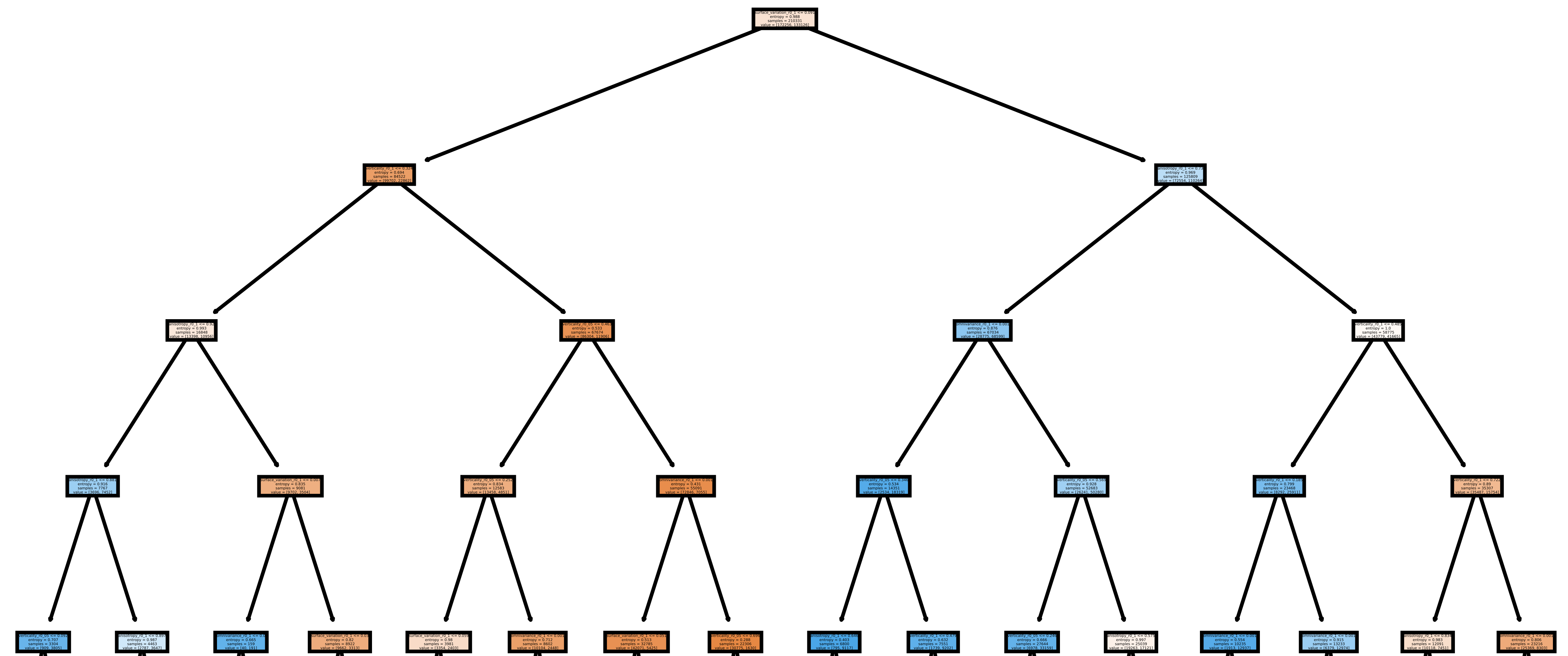
Representation of the first decision tree in the random forest.
The table below shows the results of the random forest classifier through the stratified kfolding for \(K=5\). The output is automatically generated when executing the pipeline and exported to the corresponding files. It can also be visualized in the log file that can be printed in real time during execution to monitor the pipeline’s processing.
OA |
P |
R |
F1 |
IoU |
wP |
wR |
wF1 |
wIoU |
MCC |
Kappa |
|
|---|---|---|---|---|---|---|---|---|---|---|---|
mean |
83.212 |
82.959 |
82.893 |
82.925 |
70.891 |
83.198 |
83.212 |
83.203 |
71.298 |
65.852 |
65.850 |
stdev |
0.058 |
0.054 |
0.073 |
0.064 |
0.091 |
0.061 |
0.058 |
0.060 |
0.087 |
0.126 |
0.127 |
Q1 |
83.171 |
82.925 |
82.833 |
82.877 |
70.823 |
83.152 |
83.171 |
83.159 |
71.235 |
65.758 |
65.754 |
Q3 |
83.258 |
82.997 |
82.964 |
82.980 |
70.971 |
83.251 |
83.258 |
83.254 |
71.370 |
65.961 |
65.961 |
The working example on predictive pipelines will show how the trained model can be used to compute leaf-wood segmentation on other point clouds and automatically compute the evaluation of the predictions when reference data is available.
Predictive pipeline
A predictive pipeline is a pipeline that contains a pipeline that can be used
to compute predictions. Typically, a predictive pipeline wraps a sequential
pipeline that has been used for training but then exported with a
PredictivePipelineWriter component. Predictive pipelines can be
used inside sequential pipelines and they can be combined with other
components, as shown in the JSON below:
"sequential_pipeline":[
    {
        "predict": "PredictivePipeline",
        "model_path": "/my/pipelines/leaf_wood.pipe",
        "nn_path": null
    },
    {
        "writer": "PredictionsWriter",
        "out_preds": "*predictions.lbl"
    }
]
In the JSON example above, the defined sequential pipeline loads a predictive
pipeline from /my/pipelines/leaf_wood.pipe and then uses it to compute
a leaf-wood segmentation on the input point cloud. Afterwards, the
computed predictions are exported to a single-column text file representing
the predicted labels predictions.lbl. Alternatively, the `nn_path`
element can be used to specify the path to a neural network (typically stored
as a .keras file). This specification is useful when loading a predictive
pipeline that deserializes a deep learning model whose path to the neural
network has changed, i.e., the one stored during serialization is no longer
available.
The arguments that can be specified through a JSON to build a
PredictivePipelineWriter are detailed below:
Arguments
- –
out_pipeline The output path where the serialized pipeline will be exported.
- –
include_writer Whether to include writers in the predictive pipeline.
- –
include_imputer Whether to include imputers in the predictive pipeline.
- –
include_feature_transformer Whether to include feature transformers in the predictive pipeline.
- –
include_miner Whether to include data miners in the predictive pipeline.
- –
include_class_transformer Whether to include class transformers in the predictive pipeline.
- –
include_clustering Whether to include clustering components in the predictive pipeline.
- –
ignore_predictions When set to
false, it means that the predictive pipeline must yield predictions when called or it will be considered a failed call. When set totrue, the predictive pipeline does not necessarily yield predictions. Usingtruemay be useful to generate data mining pipelines with feature transforming operations and package them into a predictive pipeline to be applied later on. For example, a standardization model can be fit once to the original dataset and then be applied with the same mean and standard deviation to different point clouds of the same dataset.
Working example
The JSON below provides an example of a predictive pipeline used inside a
sequential pipeline in a real use-case scenario. The predictions are computed
for two different input point clouds specified in in_pcloud and exported
using the two output prefixes specified in out_pcloud.
{
  "in_pcloud": [
    "test_data/QuePet_BR01_01_2019-07-03_q2_TLS-on_c.laz",
    "test_data/QueRub_KA11_09_2019-09-03_q2_TLS-on_c_t.laz"
  ],
  "out_pcloud": [
    "out/prediction/QuePet_BR01_kbest_RF/QuePet_BR01/*",
    "out/prediction/QuePet_BR01_kbest_RF/QueRub_KA11_09/*"
  ],
  "sequential_pipeline": [
    {
      "predict": "PredictivePipeline",
      "model_path": "out/training/QuePet_BR01_kbest_RF/pipe/LeafWood_Training_RF.pipe"
    },
    {
      "writer": "PredictionsWriter",
      "out_preds": "*predictions.lbl"
    },
    {
      "writer": "ClassifiedPcloudWriter",
      "out_pcloud": "*predicted.las"
    },
    {
      "eval": "ClassificationEvaluator",
      "class_names": ["wood", "leaf"],
      "metrics": ["OA", "P", "R", "F1", "IoU", "wP", "wR", "wF1", "wIoU", "MCC", "Kappa"],
      "class_metrics": ["P", "R", "F1", "IoU"],
      "report_path": "*report/global_eval.log",
      "class_report_path": "*report/class_eval.log",
      "confusion_matrix_report_path" : "*report/confusion_matrix.log",
      "confusion_matrix_plot_path" : "*plot/confusion_matrix.svg",
      "class_distribution_report_path": "*report/class_distribution.log",
      "class_distribution_plot_path": "*plot/class_distribution.svg"
    }
  ]
}
The sequential pipeline consists of fours components. First, the predictive pipeline is loaded and used to compute leaf-wood segmentation on the input point cloud. Then, the predicted labels are exported to a text file named predictions.lbl. Afterwards, a point cloud with the predictions, the references, and a binary mask (successfully classified or not) is exported. Finally, an evaluator component is used to evaluate the results. Consequently, a class-wise evaluation, a confusion matrix, and an analysis of the classes distribution are exported. The evaluator considers many metrics like the Overall Accuracy (OA), or the Matthews Correlation Coefficient (MCC).
The figure below represents a visualization of the binary mask that highlights
the successfully classified points in gray color and the misclassified points
in red color. The point cloud with the mask is automatically generated by the
ClassifiedPcloudWriter component.
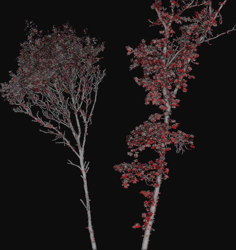
The success (gray) and fail (red) color map on two segmented trees. The left tree is the same tree used to train the model and yields better results. The right tree is from a different specie with different vegetation patterns and yields worse results.