Random forest for point-wise classification in the Hessigheim March2018 dataset
Data
The point clouds used in this example are available in the official webpage of the dataset.
JSON
The many JSON files and the bash script used to launch them in the FinisTerrae-III supercomputer of the Galicia supercomputing center (CESGA) are shown below. Note that the bash script for the FinisTerra-III is written to work with a slurm workload manager.
Data mining JSON
The JSON below can be used to compute geometric and height features as well as smoothed features derived from reflectance and color information.
{
  "in_pcloud": [
    "/mnt/netapp2/Store_uscciaep/lidar_data/hessigheim/data/Mar18_train.laz",
    "/mnt/netapp2/Store_uscciaep/lidar_data/hessigheim/data/Mar18_val.laz"
  ],
  "out_pcloud": [
    "/mnt/netapp2/Store_uscciaep/lidar_data/hessigheim/vl3d/mined/Mar18_train_mined_*",
    "/mnt/netapp2/Store_uscciaep/lidar_data/hessigheim/vl3d/mined/Mar18_val_mined_*"
  ],
  "sequential_pipeline": [
    {
      "miner": "HSVFromRGB",
      "hue_unit": "radians",
      "frenames": ["HSV_Hrad", "HSV_S", "HSV_V"]
    },
    {
      "miner": "HeightFeatures",
      "support_chunk_size": 200,
      "support_subchunk_size": 20,
      "pwise_chunk_size": 10000,
      "nthreads": 10,
      "neighborhood": {
        "type": "Rectangular2D",
        "radius": 50.0,
        "separation_factor": 0.35
      },
      "outlier_filter": null,
      "fnames": ["floor_distance"]
    },
    {
      "miner": "SmoothFeatures",
      "chunk_size": 1000000,
      "subchunk_size": 1000,
      "neighborhood": {
        "type": "sphere",
        "radius": 0.25
      },
      "input_fnames": ["Reflectance", "HSV_Hrad", "HSV_S", "HSV_V"],
      "fnames": ["mean"],
      "nthreads": 24
    },
    {
      "miner": "SmoothFeatures",
      "chunk_size": 1000000,
      "subchunk_size": 1000,
      "neighborhood": {
        "type": "sphere",
        "radius": 1.0
      },
      "input_fnames": ["Reflectance", "HSV_Hrad", "HSV_S", "HSV_V"],
      "fnames": ["mean"],
      "nthreads": 16
    },
    {
      "miner": "SmoothFeatures",
      "chunk_size": 1000000,
      "subchunk_size": 1000,
      "neighborhood": {
        "type": "sphere",
        "radius": 3.0
      },
      "input_fnames": ["Reflectance", "HSV_Hrad", "HSV_S", "HSV_V"],
      "fnames": ["mean"],
      "nthreads": 12
    },
    {
      "miner": "GeometricFeatures",
      "radius": 0.125,
      "fnames": ["linearity", "planarity", "sphericity", "surface_variation", "omnivariance", "verticality", "anisotropy", "eigenentropy", "eigenvalue_sum"]
    },
    {
      "miner": "GeometricFeatures",
      "radius": 0.25,
      "fnames": ["linearity", "planarity", "sphericity", "surface_variation", "omnivariance", "verticality", "anisotropy", "eigenentropy", "eigenvalue_sum"]
    },
    {
      "miner": "GeometricFeatures",
      "radius": 0.5,
      "fnames": ["linearity", "planarity", "sphericity", "surface_variation", "omnivariance", "verticality", "anisotropy", "eigenentropy", "eigenvalue_sum"]
    },
    {
      "miner": "GeometricFeatures",
      "radius": 0.75,
      "fnames": ["linearity", "planarity", "sphericity", "surface_variation", "omnivariance", "verticality", "anisotropy", "eigenentropy", "eigenvalue_sum"]
    },
    {
      "miner": "GeometricFeatures",
      "radius": 1.0,
      "fnames": ["linearity", "planarity", "sphericity", "surface_variation", "omnivariance", "verticality", "anisotropy", "eigenentropy", "eigenvalue_sum"]
    },
    {
      "miner": "GeometricFeatures",
      "radius": 2.0,
      "fnames": ["linearity", "planarity", "sphericity", "surface_variation", "omnivariance", "verticality", "anisotropy", "eigenentropy", "eigenvalue_sum"]
    },
    {
      "miner": "GeometricFeatures",
      "radius": 3.0,
      "fnames": ["linearity", "planarity", "sphericity", "surface_variation", "omnivariance", "verticality", "anisotropy", "eigenentropy", "eigenvalue_sum"]
    },
    {
      "miner": "GeometricFeatures",
      "radius": 5.0,
      "fnames": ["linearity", "planarity", "sphericity", "surface_variation", "omnivariance", "verticality", "anisotropy", "eigenentropy", "eigenvalue_sum"]
    },

    {
      "writer": "Writer",
      "out_pcloud": "*feats.las"
    }
  ]
}
Training JSON
The training JSON considers geometric, height, reflectance, and color features to train a random forest classifier with an auto validation training strategy. The trained model is exported together with the data imputation components to a predictive pipeline.
{
  "in_pcloud": [
    "/mnt/netapp2/Store_uscciaep/lidar_data/hessigheim/vl3d/mined/Mar18_train_mined_feats.las"
  ],
  "out_pcloud": [
    "/mnt/netapp2/Store_uscciaep/lidar_data/hessigheim/vl3d/rf_hessig/*"
  ],
  "sequential_pipeline": [
    {
      "imputer": "UnivariateImputer",
      "fnames": [
        "Reflectance", "HSV_Hrad", "HSV_S", "HSV_V",
        "Reflectance_mean_r0.25", "Reflectance_mean_r1.0", "Reflectance_mean_r3.0",
        "HSV_Hrad_mean_r0.25", "HSV_Hrad_mean_r1.0", "HSV_Hrad_mean_r3.0",
        "HSV_S_mean_r0.25", "HSV_S_mean_r1.0", "HSV_S_mean_r3.0",
        "HSV_V_mean_r0.25", "HSV_V_mean_r1.0", "HSV_V_mean_r3.0",
        "floor_distance_r50.0_sep0.35", "linearity_r0.125", "planarity_r0.125",
        "sphericity_r0.125", "surface_variation_r0.125", "omnivariance_r0.125",
        "verticality_r0.125", "anisotropy_r0.125", "eigenentropy_r0.125",
        "eigenvalue_sum_r0.125", "linearity_r0.25", "planarity_r0.25",
        "sphericity_r0.25", "surface_variation_r0.25", "omnivariance_r0.25",
        "verticality_r0.25", "anisotropy_r0.25", "eigenentropy_r0.25",
        "eigenvalue_sum_r0.25", "linearity_r0.5", "planarity_r0.5",
        "sphericity_r0.5", "surface_variation_r0.5", "omnivariance_r0.5",
        "verticality_r0.5", "anisotropy_r0.5", "eigenentropy_r0.5",
        "eigenvalue_sum_r0.5", "linearity_r0.75", "planarity_r0.75",
        "sphericity_r0.75", "surface_variation_r0.75", "omnivariance_r0.75",
        "verticality_r0.75", "anisotropy_r0.75", "eigenentropy_r0.75",
        "eigenvalue_sum_r0.75", "linearity_r1.0", "planarity_r1.0",
        "sphericity_r1.0", "surface_variation_r1.0", "omnivariance_r1.0",
        "verticality_r1.0", "anisotropy_r1.0", "eigenentropy_r1.0",
        "eigenvalue_sum_r1.0", "linearity_r2.0", "planarity_r2.0",
        "sphericity_r2.0", "surface_variation_r2.0", "omnivariance_r2.0",
        "verticality_r2.0", "anisotropy_r2.0", "eigenentropy_r2.0",
        "eigenvalue_sum_r2.0", "linearity_r3.0", "planarity_r3.0",
        "sphericity_r3.0", "surface_variation_r3.0", "omnivariance_r3.0",
        "verticality_r3.0", "anisotropy_r3.0", "eigenentropy_r3.0",
        "eigenvalue_sum_r3.0", "linearity_r5.0", "planarity_r5.0",
        "sphericity_r5.0", "surface_variation_r5.0", "omnivariance_r5.0",
        "verticality_r5.0", "anisotropy_r5.0", "eigenentropy_r5.0",
        "eigenvalue_sum_r5.0"
      ],
      "target_val": "NaN",
      "strategy": "mean",
      "constant_val": 0
    },
    {
      "train": "RandomForestClassifier",
      "fnames": [
        "Reflectance", "HSV_Hrad", "HSV_S", "HSV_V",
        "Reflectance_mean_r0.25", "Reflectance_mean_r1.0", "Reflectance_mean_r3.0",
        "HSV_Hrad_mean_r0.25", "HSV_Hrad_mean_r1.0", "HSV_Hrad_mean_r3.0",
        "HSV_S_mean_r0.25", "HSV_S_mean_r1.0", "HSV_S_mean_r3.0",
        "HSV_V_mean_r0.25", "HSV_V_mean_r1.0", "HSV_V_mean_r3.0",
        "floor_distance_r50.0_sep0.35", "linearity_r0.125", "planarity_r0.125",
        "sphericity_r0.125", "surface_variation_r0.125", "omnivariance_r0.125",
        "verticality_r0.125", "anisotropy_r0.125", "eigenentropy_r0.125",
        "eigenvalue_sum_r0.125", "linearity_r0.25", "planarity_r0.25",
        "sphericity_r0.25", "surface_variation_r0.25", "omnivariance_r0.25",
        "verticality_r0.25", "anisotropy_r0.25", "eigenentropy_r0.25",
        "eigenvalue_sum_r0.25", "linearity_r0.5", "planarity_r0.5",
        "sphericity_r0.5", "surface_variation_r0.5", "omnivariance_r0.5",
        "verticality_r0.5", "anisotropy_r0.5", "eigenentropy_r0.5",
        "eigenvalue_sum_r0.5", "linearity_r0.75", "planarity_r0.75",
        "sphericity_r0.75", "surface_variation_r0.75", "omnivariance_r0.75",
        "verticality_r0.75", "anisotropy_r0.75", "eigenentropy_r0.75",
        "eigenvalue_sum_r0.75", "linearity_r1.0", "planarity_r1.0",
        "sphericity_r1.0", "surface_variation_r1.0", "omnivariance_r1.0",
        "verticality_r1.0", "anisotropy_r1.0", "eigenentropy_r1.0",
        "eigenvalue_sum_r1.0", "linearity_r2.0", "planarity_r2.0",
        "sphericity_r2.0", "surface_variation_r2.0", "omnivariance_r2.0",
        "verticality_r2.0", "anisotropy_r2.0", "eigenentropy_r2.0",
        "eigenvalue_sum_r2.0", "linearity_r3.0", "planarity_r3.0",
        "sphericity_r3.0", "surface_variation_r3.0", "omnivariance_r3.0",
        "verticality_r3.0", "anisotropy_r3.0", "eigenentropy_r3.0",
        "eigenvalue_sum_r3.0", "linearity_r5.0", "planarity_r5.0",
        "sphericity_r5.0", "surface_variation_r5.0", "omnivariance_r5.0",
        "verticality_r5.0", "anisotropy_r5.0", "eigenentropy_r5.0",
        "eigenvalue_sum_r5.0"
      ],
      "training_type": "autoval",
      "random_seed": null,
      "shuffle_points": true,
      "num_folds": 5,
      "model_args": {
        "n_estimators": 360,
        "criterion": "entropy",
        "max_depth": 25,
        "min_samples_split": 32,
        "min_samples_leaf": 8,
        "min_weight_fraction_leaf": 0.0,
        "max_features": "sqrt",
        "max_leaf_nodes": null,
        "min_impurity_decrease": 0.0,
        "bootstrap": true,
        "oob_score": false,
        "n_jobs": 32,
        "warm_start": false,
        "class_weight": "balanced_subsample",
        "ccp_alpha": 0.0,
        "max_samples": 0.3
      },
      "autoval_metrics": ["OA", "P", "R", "F1", "IoU", "wP", "wR", "wF1", "wIoU", "MCC", "Kappa"],
      "stratkfold_report_path": "*report/RF_stratkfold_report.log",
      "stratkfold_plot_path": "*plot/RF_stratkfold_plot.svg",
      "importance_report_path": "*report/RF_importance.log",
      "importance_report_permutation": false,
      "decision_plot_path": "*plot/RF_decision.svg",
      "decision_plot_trees": 3,
      "decision_plot_max_depth": 5
    },
    {
      "writer": "PredictivePipelineWriter",
      "out_pipeline": "*pipe/rf_hessig.pipe",
      "include_writer": false,
      "include_imputer": true,
      "include_feature_transformer": false,
      "include_miner": false
    }
  ]
}
Classification JSON
The classification JSON applies the predictive pipeline to previously unseen data to assess the model and the uncertainties.
{
  "in_pcloud": [
    "/mnt/netapp2/Store_uscciaep/lidar_data/hessigheim/vl3d/mined/Mar18_val_mined_feats.las"
  ],
  "out_pcloud": [
    "/mnt/netapp2/Store_uscciaep/lidar_data/hessigheim/vl3d/rf_hessig/validation/*"
  ],
  "sequential_pipeline": [
    {
      "predict": "PredictivePipeline",
      "model_path": "/mnt/netapp2/Store_uscciaep/lidar_data/hessigheim/vl3d/rf_hessig/pipe/rf_hessig.pipe"
    },
    {
      "writer": "ClassifiedPcloudWriter",
      "out_pcloud": "*predicted.las"
    },
    {
      "eval": "ClassificationEvaluator",
      "class_names": ["Low vegetation", "Impervious surface", "Vehicle", "Urban furniture", "Roof", "Facade", "Shrub", "Tree", "Soil/Gravel", "Vertical surface", "Chimney"],
      "metrics": ["OA", "P", "R", "F1", "IoU", "wP", "wR", "wF1", "wIoU", "MCC", "Kappa"],
      "class_metrics": ["P", "R", "F1", "IoU"],
      "report_path": "*report/global_eval.log",
      "class_report_path": "*report/class_eval.log",
      "confusion_matrix_report_path" : "*report/confusion_matrix.log",
      "confusion_matrix_plot_path" : "*plot/confusion_matrix.svg",
      "class_distribution_report_path": "*report/class_distribution.log",
      "class_distribution_plot_path": "*plot/class_distribution.svg"
    },
    {
        "eval": "ClassificationUncertaintyEvaluator",
        "class_names": ["Low vegetation", "Impervious surface", "Vehicle", "Urban furniture", "Roof", "Facade", "Shrub", "Tree", "Soil/Gravel", "Vertical surface", "Chimney"],
        "include_probabilities": true,
        "include_weighted_entropy": true,
        "include_clusters": true,
        "weight_by_predictions": false,
        "num_clusters": 10,
        "clustering_max_iters": 128,
        "clustering_batch_size": 1000000,
        "clustering_entropy_weights": true,
        "clustering_reduce_function": "mean",
        "gaussian_kernel_points": 256,
        "report_path": "*uncertainty/uncertainty.las",
        "plot_path": "*uncertainty/"
    }
  ]
}
Bash script for slurm
The bash script below can be used at CESGA to queue a node with 32 cores and 246 GB RAM to execute the data mining, training, and classification JSONs with a maximum expected time of 48 hours.
#!/bin/bash
#SBATCH -N 1
#SBATCH -n 1
#SBATCH -c 32
#SBATCH -t 48:00:00
#SBATCH --mem 246GB
#SBATCH --mail-type=begin
#SBATCH --mail-type=end
#SBATCH [email protected]

# Author: Alberto M. Esmoris Pena
#
# Brief:    Script to use VL3D framework at CESGA'S FT-III
#           For urban semantic segmentation on the Hessigheim
#           dataset.


# ---  VARIABLES  --- #
# ------------------- #
VL3D_DIR='/home/usc/ci/aep/git/virtualearn3d/'
VL3D_SCRIPT='/home/usc/ci/aep/git/virtualearn3d/vl3d.py'
MINE_SPEC='/home/usc/ci/aep/git/virtualearn3d/cesga/hessigheim/rf_hessig_mine.json'
TRAINING_SPEC='/home/usc/ci/aep/git/virtualearn3d/cesga/hessigheim/rf_hessig_train.json'
PREDICTIVE_SPEC='/home/usc/ci/aep/git/virtualearn3d/cesga/hessigheim/rf_hessig_predict.json'

# ---  EXECUTION  --- #
# ------------------- #
# LOAD MODULES
module load cesga/system python/3.10
conda activate /mnt/netapp2/Store_uscciaep/vl3d_conda_env

# RUN SCRIPTS
cd "${VL3D_DIR}"
srun python ${VL3D_SCRIPT} --pipeline ${MINE_SPEC}
srun python ${VL3D_SCRIPT} --pipeline ${TRAINING_SPEC}
srun python ${VL3D_SCRIPT} --pipeline ${PREDICTIVE_SPEC}
Quantification
The table below shows the class-wise evaluation metrics.
CLASS |
P |
R |
F1 |
IoU |
|---|---|---|---|---|
Low vegetation |
82.735 |
92.883 |
87.516 |
77.803 |
Impervious surface |
86.374 |
90.859 |
88.560 |
79.468 |
Vehicle |
90.981 |
25.079 |
39.319 |
24.470 |
Urban furniture |
51.167 |
52.387 |
51.770 |
34.925 |
Roof |
94.533 |
89.498 |
91.947 |
85.094 |
Facade |
66.081 |
87.050 |
75.130 |
60.166 |
Shrub |
63.518 |
50.608 |
56.333 |
39.211 |
Tree |
92.247 |
96.023 |
94.097 |
88.853 |
Soil/Gravel |
78.362 |
14.883 |
25.015 |
14.295 |
Vertical surface |
92.356 |
47.138 |
62.418 |
45.368 |
Chimney |
97.081 |
48.099 |
64.327 |
47.414 |
The table below shows the global evaluation metrics.
OA |
P |
R |
F1 |
IoU |
wP |
wR |
wF1 |
wIoU |
MCC |
Kappa |
|---|---|---|---|---|---|---|---|---|---|---|
85.281 |
81.403 |
63.137 |
66.948 |
54.279 |
85.417 |
85.281 |
83.986 |
74.934 |
81.805 |
81.663 |
Visualization
The figure below shows the results of the previously explained pipelines.
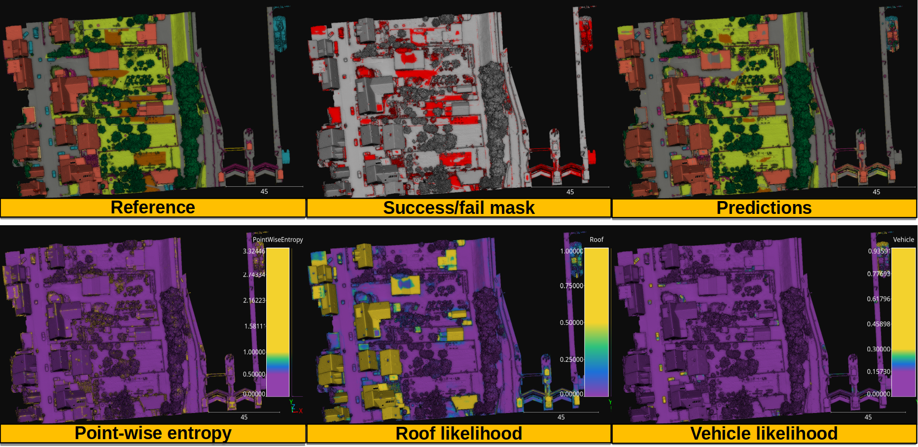
Visualization of the reference and predictions together with the binary fail/success mask. Also, the point-wise entropy and the likelihood for the roof and vehicle classes.
Application
This example has two main applications:
Baseline model for urban semantic segmentation in 3D point clouds with machine learning.
Exploring the adequateness of a given set of features for urban semantic segmentation. Since the machine learning model does not derive features but uses given features, it can be used to assess how well different sets of features perform.